Bay Area Tutoring

Oct 13

A mnemonic for remembering values on the unit circle

By Tutor GuyNo Comments

In an earlier post, I told you that you must memorize the values on the unit circle if you want to be great at trigonometry. So let’s say that you have taken my advice, but on a test you have a big brain cramp and you forget the values. Here’s a trick that will help you fill in the values in the first quadrant. The five angles in the first quadrant are 0°, 30°, 45°, 60°, and 90°. And the sines of these angles just happen to be:

$\underline{ \qquad \theta \qquad \sin \theta \qquad \qquad \qquad}$

$0 \textdegree \qquad \; \; 0 \qquad =\dfrac{\sqrt{0}}{2}$

$30 \textdegree \qquad \dfrac{1}{2} \qquad = \dfrac{\sqrt{1}}{2}$

$45 \textdegree \qquad \dfrac{\sqrt{2}}{2} \quad = \dfrac{\sqrt{2}}{2}$

$60 \textdegree \qquad \dfrac{\sqrt{3}}{2} \quad = \dfrac{\sqrt{3}}{2}$

$90 \textdegree \qquad 1 \qquad = \dfrac{\sqrt{4}}{2}$

Do you see the pattern in the last column? The sines increase from

$\dfrac{\sqrt{0}}{2}$ to $\dfrac{\sqrt{4}}{2}$

That’s an easy pattern to remember even during the worst brain cramp. Why does it work? It’s just a coincidence. But if you use this pattern, you can fill in the sine values in the first quadrant. Then the cosine values are the same in reverse order. Once you’ve completed the first quadrant, you can fill in the rest of the unit circle by using reference angles. Now you have a completed unit circle!

Algebra 2, Precalc/Trig

math, math homework, trig, unit circle

Oct 06

Identifying a probability distribution II—normal, t and chi-square

By Tutor GuyNo Comments

Often the first step in determining the probability of an event is determining the probability distribution to which the event belongs. Good statisticians can identify the correct distribution right away; if you learn some simple rules, you can specify the correct distribution just like the experts. In this post, I describe how to identify the three most common continuous distributions: normal, t and chi-square.

Requirements for a normal distribution

Many times you will be told when a distribution is normally distributed. When you are conducting hypotheses tests, you will often assume that the distribution is normal (or at least approximately normal) when the following conditions hold:

The standard deviation (σ) of the population is known
The sample size (n) is ≥30
The statistic you are measuring is the sample mean

Requirements for a t distribution

If you are performing a hypothesis test and you are measuring the sample mean, you will need to use a t distribution instead of a normal distribution if either of the following conditions holds:

The standard deviation (σ) of the population is not known.
The sample size (n) is < 30

Requirements for a chi-square (Χ²) distribution

There are numerous situations where a chi-square distribution is indicated. In a first year stats class, you will use chi-square distributions when you are performing a contingency test, a goodness-of-fit test or a test of homogeneity.

Statistics

Sep 29

Identifying a probability distribution I—binomial and geometric

By Tutor GuyNo Comments

Often the first step in determining the probability of an event is determining the probability distribution to which the event belongs. Good statisticians can identify the correct distribution right away; if you learn some simple rules, you can specify the correct distribution just like the experts. In this post, I describe how to identify the two most common discrete distributions: binomial and geometric.

Requirements for a binomial distribution

There are a fixed number, n, of trials.
All trials are independent.
The probability, p, of success in each trial is a constant.
We are interested in the number of successes in the n trials.

If these conditions are met, you have a binomial distribution. Here’s an example question: “A manufacturing process produces widgets with a known defect rate of 2%. If 100 widgets are selected at random, what is the probability that exactly three are defective?” Here, the 100 selected widgets represent the 100 trials (a fixed number). The probability of finding a defective widget in each trial is a constant 2%. We are looking for the probability of finding three defective widgets (we are counting the number of times we find a defective widget). So we know we have a binomial distribution.

Note that if the population is finite, the probability of success will change slightly each time we select an item. That means we do not have a binomial distribution. However, if the population is large enough, the probability does not change very much and we can approximate the problem with a binomial distribution. A common rule of thumb for using the approximate binomial is to require that the population size, N, be at least ten times larger than the sample size, n.

Requirement for a geometric distribution

All trials are independent.
The probability, p, of success in each trial is a constant.
We count the number of trials until the first success.

If these conditions are met, you have a geometric distribution. Note that the conditions are similar to the binomial distribution conditions, but the number of trials is not fixed and we are not counting the number of successes. Here’s an example question: “A manufacturing process produces widgets with a known defect rate of 2%. What is the probability that 100 good widgets are inspected before the first defective widget is found?” Note that this question looks somewhat similar to the previous example. But this time we have phrased the question in a way that leads to a geometric distribution.

Statistics

binomial, geometric, probability distributions, statistics

Sep 22

Using the reciprocal key on your calculator

By Tutor GuyNo Comments

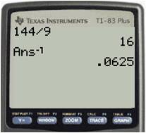
Your graphing calculator has a reciprocal key on it, designated as $x^{-1}$ . It’s the easiest way to find the reciprocal of a number on your screen. Just press the key, and then Enter.

The reciprocal key is also a great way to do calculations of resistors in parallel or capacitors in series. For example, find the equivalent resistance of a circuit that has a 10 Ω and a 15 Ω resistor in parallel. Simply enter it this way into the calculator to find the answer is 6 Ω.

Algebra 2, Calculator, Physics, Precalc/Trig

math, math homework, reciprocals

Sep 15

Factoring the difference of two squares

By Tutor GuyNo Comments

You will spend a lot of time in algebra (and courses beyond) factoring polynomials into linear and quadratic terms. There are some special polynomials that occur so frequently that you should recognize them on sight so that you know the method for factoring them. The most common is the binomial of the form $a^2-b^2$ . This is called the difference of two squares because both terms are perfect squares and you are subtracting (finding the difference between) the two terms.

Some examples of this binomial are $x^2-4$ , $9x^4-16y^2$ and $121y^2z^2-25w^4a^6b^{12}$ . Note that in each case, both terms are perfect squares.

It is very easy to factor these expressions—you can do it by inspection. The rule is simple and you must memorize it: $a^2-b^2=(a+b)(a-b)$ . Once you determine that an expression is the difference of two squares, you can write out its factors immediately. Let’s see how it works with the three examples given above:

$x^2-4=(x+2)(x-2)$

$9x^4-16y^2=(3x^2+4y)(3x^2-4y)$

$121y^2z^2-25w^4a^6b^{12}=(11yz+5w^2a^3b^6)(11yz-5w^2a^3b^6)$

It’s really that easy once you learn the format. Of course it doesn’t matter what order you write the two factors, so $x^2-4=(x-2)(x+2)$ is also correct.

One other important point: this factoring rule works in reverse, too! If you have to distribute (multiply out) two factors and you see they are in the form of $(a+b)(a-b)$ , you should recognize that this gives the difference of two squares: $a^2-b^2$ . You can do this immediately, without multiplying out every term. Learning this formula will save you lots of time.

Algebra 1, Algebra 2, Precalc/Trig

difference of two squares, factoring, math, math homework

Sep 08

How to manage projectile motion problems

By Tutor GuyNo Comments

In two-dimensional kinematics problems (for example, a ball thrown forward or a missile fired through the air), keep the horizontal ( $x$ ) and vertical ( $y$ ) directions separate. The motions in each direction are independent of each other, so you can work them separately.

In the $x$ direction, the velocity will be constant because there is no horizontal force on the object (ignoring air resistance). In the $y$ direction, you need to include the acceleration term due to gravity.

If the object’s initial velocity is not totally horizontal or totally vertical, you need to find the horizontal and vertical components first. If the initial velocity is $v_0$ and the initial angle is θ, then the two velocity components are:

$v_x=v_0 \cos \theta$
$v_y=v_0 \sin \theta$

Then the position functions in each direction are as follows:

$S_x=v_x t + S_{0x}$

$S_y=-\frac{1}{2}{}gt^2+v_yt+s_{0y}$

Physics

components, kinematics, physics

Sep 01

Graphing rational functions—4. Drawing the graph

By Tutor GuyNo Comments

In previous posts, I described the steps you follow to analyze a rational function. If you follow these steps, you can be a rational function superstar too. In this post, I put all the pieces together to show how you use the information you’ve obtained to plot the graph. [For details on how to execute the various steps, please see other posts on this website.]

Example: Graph the following rational function.

$f(x)=\dfrac{2x^3-16x^2+38x-24}{x^3-4x^2+x+6}$

Solution: We break this into many steps.

1. Find the $y$ -intercept:

$f(0)=\dfrac{-24}{6}=-4$

2. Fully factor the function:

$f(x)=\dfrac{2x^3-16x^2+38x-24}{x^3-4x^2+x+6}=\dfrac{2(x-1)(x-3)(x-4)}{(x+1)(x-2)(x-3)}$

3. Find the vertical asymptotes, if any:

The vertical asymptotes are at $x=-1$ and $x=2$ .

4.Find the $x$ -intercept(s), if any:

$f(x)=0$ @ $x=1$ and $x=4$

5. Find the hole(s), if any:

There is a hole at the point $(3,-1)$

6. Find the horizontal or oblique asymptote, if any, or characterize the end behavior:

The horizontal asymptote is at $y=2$

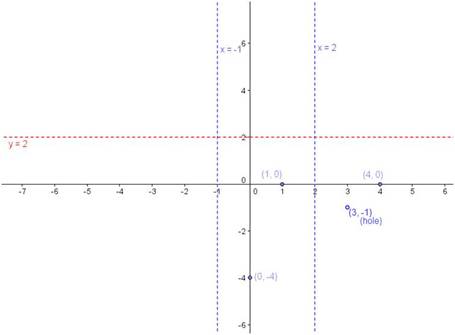
7. Place all of this information on the graph:

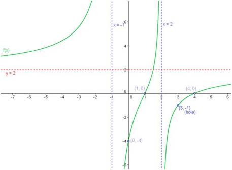
8. Use all the information you have plotted to complete the graph of the function:

Algebra 2, Precalc/Trig

math, math homework, rational functions

Aug 25

Graphing rational functions—3. Finding horizontal or oblique asymptotes

By Tutor GuyNo Comments

In a previous post, I listed the steps you need to follow to analyze and graph a rational function. In this post, I show you how to find the horizontal or oblique asymptotes, if they exist. If there are no horizontal or oblique asymptotes, then you can determine the end behavior of the function. [Check other posts on this website for other steps in analyzing and graphing a rational function.]

The horizontal and oblique asymptotes, if they exist, tell you the end behavior of the function. That is, they describe what the function is doing as $x$ goes to ±∞. In order to determine the end behavior, examine the degrees of the polynomials in the numerator and denominator. There are four possible cases:

Case 1: The degree of the denominator is greater than the degree of the numerator.

When the denominator has the higher degree, the denominator grows much faster than the numerator as $x$ gets very large. Like all fractions, as the denominator gets very large, the fraction gets very small and approaches zero. So the asymptote is $y=0$ .

Example 1: Find the end behavior for the following rational function:

$f(x)=\dfrac{x^2+3x+2}{x^3+4x^2+x-6}$

Solution: Because the degree of the numerator is $2$ and the degree of the denominator is $3$ , this function has a horizontal asymptote $y=0$ .

Case 2: The degree of the denominator is equal to the degree of the numerator.

When the degrees of the numerator and denominator are the same, the function approaches a finite non-zero number. This number is the ratio of the leading coefficients of the two polynomials and this is the value of the horizontal asymptote.

Example 2: Find the end behavior for the following rational function:

$f(x)=\dfrac{6x^2+7x-4}{5x^2-4x-6}$

Solution: Because the degree of the numerator and denominator are the same, this function has a horizontal asymptote. Divide the leading coefficients ( $6$ and $5$ ) and the horizontal asymptote is $y=6/5$ .

Case 3: The degree of the numerator is exactly one higher than the degree of the denominator.

In this case, there is an oblique asymptote (called a slant asymptote in some textbooks). To find the asymptote, divide the denominator into the numerator using long division. The quotient is the oblique asymptote. (Ignore the remainder; it has no effect on the asymptote.)

Example 3: Find the end behavior for the following rational function:

$f(x)=\dfrac{x^3+4x^2+x-6}{x^2+3x+2}$

Here, the numerator (degree 3) is exactly one higher than the denominator (degree 2). To find the asymptote, perform the following long division:

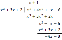
The quotient is the oblique asymptote:

$y=x+1$

Case 4: The degree of the numerator is more than one higher than the degree of the denominator.

In this case, there is no horizontal or oblique asymptote. Instead, the end behavior of the function is the same as the end behavior of a polynomial whose degree is the same as the difference between the degrees of the numerator and the denominator. For example, if the numerator is degree $5$ and the denominator is degree $2$ , the rational function will look like a cubic function as $x$ approaches ±∞.

Algebra 2, Precalc/Trig

math, math homework, rational functions

Aug 18

Graphing rational functions—2. Finding holes and vertical asymptotes

By Tutor GuyNo Comments

In a previous post, I listed the steps you need to follow to analyze and graph a rational function. In this post, I show you how to find the hole(s) and vertical asymptote(s), if they exist. [Check other posts on this website for other steps in analyzing and graphing a rational function.]

In a rational function, holes and vertical asymptotes will only occur where the denominator is equal to zero. So fully factor the function, and look for the roots of the denominator. When a factor in the denominator cancels out with a factor in the numerator, the function will have a hole where the factor equals zero. If the factor in the denominator does not cancel out with a factor in the numerator, there will be a vertical asymptote where the factor equals zero.

Example: Find the holes and vertical asymptotes, if any, for the following rational function:

$f(x)=\dfrac{x^2+3x+2}{x^3+4x^2+x-6}$

First, fully factor the function:

$f(x)=\dfrac{x^2+3x+2}{x^3+4x^2+x-6}=\dfrac{(x+1)(x+2)}{(x-1)(x+2)(x+3)}=\dfrac{(x+1)}{(x-1)(x+3)}$

The roots of the denominator are $-3$ , $-2$ and $1$ . At $x=-2$ , there is a hole. To find the “value” of the hole, evaluate the reduced function:

$f(-2)=\dfrac{(-2+1)}{(-2-1)(-2+3)}=\dfrac{-1}{-3}=\dfrac{1}{3}$

This means that when you graph the function, there will be a hole at the point $(-2, 1/3)$ .

The vertical asymptotes will be $x=-3$ and $x=1$ .

Algebra 2, Precalc/Trig

math, math homework, rational functions

Aug 11

Graphing rational functions—1. Finding x- and y- intercepts

By Tutor GuyNo Comments

In a previous post, I listed the steps you need to follow to analyze and graph a rational function. In this and subsequent posts, I will walk you through each of those steps. Usually the first step in plotting a rational function is finding the $x$ – and $y$ -intercepts. You have done this before for other functions and the process here is no different.

To find the $y$ -intercept, set $x=0$ and solve for $f(x)$ .
To find the $x$ -intercept(s), set $f(x)=0$ and solve for $x$ . Recall that a rational function is a fraction, and a fraction can only be equal to zero when its numerator is equal to zero (as long as the denominator is not also equal to zero!). So in practice, you find the $x$ -intercept(s) by setting the numerator equal to zero and solving for $x$ .

Example: Find the $x$ – and $y$ -intercepts, if any, for the following rational function:

$f(x) = \dfrac{x^3+4x^2+x-6}{x^2+3x+2}$

Finding the $y$ -intercept is very easy if the polynomials are written in standard form as above. $f(0)$ is simply the ratio of the constant terms: $\frac{-6}{2} = -3$ . If the rational function has already been factored, you need to plug zero in to each term and evaluate.

To find the $x$ -intercept (and all the other parts of the rational function), the first thing you need to do is fully factor the numerator and denominator.

$f(x)=\dfrac{x^3+4x^2+x-6}{x^2+3x+2}=\dfrac{(x-1)(x+2)(x+3)}{(x+1)(x+2)}$

From here, it is easy to see that the roots of the numerator are $-3$ , $-2$ and $1$ . When $x=-2$ , the denominator is also zero, so this is not an $x$ -intercept; it is a hole. The $x$ ‑intercepts are at $-3$ and $1$ .

Is it possible that a rational function does not have a $y$ -intercept? Yes, if the function is not defined for $x=0$ . In other words, if a rational function has either a hole or a vertical asymptote at $x=0$ , there is no $y$ -intercept.

[Check out my other posts in this section that describe how to perform the other steps when analyzing a rational function.]

Algebra 2, Precalc/Trig

math, math homework, rational functions

Tutor Guy Homework Tips