Archive

For the Physics category

Right-hand rules

No Comments


The “right-hand rule” is a valuable tool in physics to help you determine the direction of vectors and fields. When you use the right-hand rule properly, your work is a lot easier. In this post, I describe a number of right-hand rules and show you how to apply them. But first, a warning:

Never, ever use a left-hand rule!

You may already know that one use of the right-hand rule is to find the direction of the force on a positively charged particle. If you want to know the direction of the force on a negatively charged particle, you use the right-hand rule and then reverse the direction you obtain. Almost every year, I get a student who comes up with the clever idea to use a left-hand rule on negative particles. Does this work? Absolutely! So why is it a bad idea? Because once you’ve used the left-hand rule, you’ve created a muscle memory that says it is okay. And the next time you need to use a right-hand rule, you may pick up your left hand without even thinking about it and you will get the wrong result. (This is particularly true if you are right handed—you already have a pencil in your right hand, so it seems perfectly natural to use your free hand.) You won’t even realize you got the wrong answer. When I teach students the right-hand rule for the first time, I train them to sit on their left hands so they won’t be tempted to use them by mistake. After 10 or 20 times using the right-hand rule, you’ll develop a muscle memory that says “only the right hand will do” and you will be less likely to make this mistake.

  • Cross products: When you find the cross product of two vectors, the result is perpendicular to each of the original vectors. But does the resultant vector point “above” the plane of the two vectors or “below” the plane? Use the right-hand rule to determine the direction of this vector. There are a number of ways to implement this right-hand rule. I’ve seen textbooks that teach you to imagine an arrow coming out of your palm. My dad learned to contort his fingers like this, with his thumb up, his index finger pointing out and his middle finger pointing perpendicular to his palm:

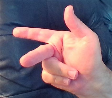
He taught this method to me, but I think it’s hard to remember which finger goes with which vector.


Here’s the technique I think works best: Let’s say you want to find the direction of \vec{u} \times \vec{v}. Point your fingers in the direction of \vec{u}.  Curl your fingers so that they point in the direction of \vec{v}.  (Find the smallest angle between \vec{u} and \vec{v}. ) Your outstretched thumb points in the direction of the cross product. Note that you may have to rotate your wrist before you curl your fingers so that they will point in the correct direction.


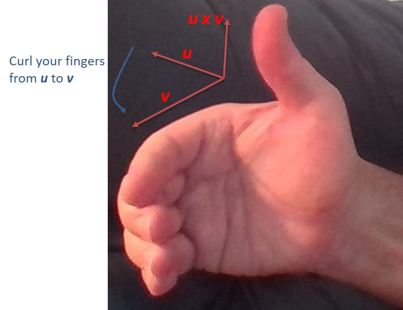
Here are some vector products where you can use the right-hand rule to determine the direction of the vector product:

\bullet \quad \vec{\tau} = \vec{r} \times \vec{F} (torque)

\bullet \quad \vec{L} = \vec{r} \times \vec{p} (angular momentum)

\bullet \quad \vec{F}_B = q\vec{v} \times \vec{B} (magnetic force on a moving charge)

\bullet \quad \vec{F}_{wire} = I\vec{\ell} \times \vec{B} (magnetic force on a wire due to a current)

Use this same rule when you are constructing coordinate axes in space. Use the rule to point the three positive axes in the correct direction given that \vec{x} \times \vec{y} = \vec{z}.

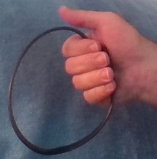
  • Magnetic field due to the current in a wire: When a current travels through a wire, it generates magnetic field lines that form concentric circles around the wire. But does the magnetic field point clockwise or counterclockwise? Use the right-hand rule to determine the direction of the field. Grip the wire with your right hand so that your thumb points in the direction of the (conventional) current. Then your fingers curl around the wire in the direction of the field. If the wire is bent into a loop, this same method tells you which direction through the loop the field points.

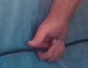
In this photo, the current is moving to the left. Point your thumb to the left, and you see the field lines are moving down behind the wire and are moving up in front of the wire.


  • Lenz’ law: When a loop of wire is placed in a location where the magnetic flux is changing, a current is induced in the wire. But in which direction is the induced current? Use a right-hand rule to determine the direction of the current. First determine the direction of the induced magnetic field predicted by Lenz’ law. If the flux is increasing through the loop the induced magnetic field has to point in the direction opposite the flux. If the flux is decreasing, the induced field points in the same direction as the flux. Now wrap your fingers around the wire so that they are pointing in the direction of this induced flux. Your thumb points in the direction of the induced current. Note that this right-hand rule is essentially the reverse of the previous rule.

In this photo, we have determined the induced flux must point out of the page towards our point of view. We curl our fingers to show this direction and we see the induced emf and induced current will be counterclockwise.


  • Ampere’s law: The loop integral \oint \vec{B} \cdot d \vec{s} around an Amperian loop is proportional to the net current through the loop. But in which direction through the loop is the current positive? Use a right-hand rule to determine the direction of positive current. Curl your fingers around the loop in the direction of integration. Your thumb points in the direction of positive current.

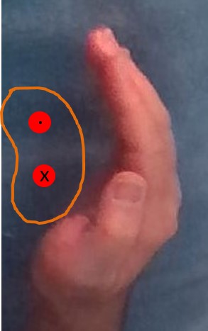
Our Amperian loop is shown in orange in this photo. The two red circles represent current-carrying wires. The top wire has current coming out of the page and the bottom wire has current flowing into the page.  We choose to integrate in a counterclockwise direction. Curl your fingers in that direction and your thumb points out of the page (towards your point of view). Therefore the top wire will be assigned a positive current and the bottom wire will be assigned a negative current in order to apply Ampere’s law.

How does the speed of light relate to Maxwell’s equations?

No Comments


You may have seen in your physics class that the speed of light can be calculated from the permittivity of free space, \varepsilon_0 
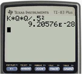
, and the permeability of free space, \mu_0 , as follows:

c = \dfrac{1}{\sqrt{\varepsilon_0 \mu_0}}

where  \varepsilon_0 = 8.85 \; C^2/N \cdot m^2 and  \mu_0 = 4 \pi \cdot 10^{-7} \; T \cdot m/A .

Sure enough, plug the numbers into your calculator and you do get the correct value for the speed of light. It’s a very famous result, and helped convince Maxwell that light is an electromagnetic wave. But the units just don’t seem to work out, do they? Well, actually they do. Let’s do the dimensional analysis. We want to show the following:

\dfrac{m}{s} = \dfrac{1}{\sqrt{\dfrac{C^2}{N \cdot m^2} \times \dfrac{T \cdot m}{A}}} \; \; (1)

From the equation for the magnetic force on a charged particle:

F = qvB \; \rightarrow \; B = \dfrac{F}{qv}

If we express this equation in terms of its units and simplify we have

T = \dfrac{N}{C \cdot m/s} = \dfrac{N \cdot s}{C \cdot m}

We also note that 1 A = 1 C/s, so we substitute for T and A in equation (1) above to get:

\dfrac{m}{s} = \dfrac{1}{\sqrt{\dfrac{C^2}{N \cdot m^2} \times \dfrac{N \cdot s}{C \cdot m} \dfrac{m \cdot s}{C}}} = \dfrac{1}{\sqrt{\dfrac{s^2}{m^2}}} = \dfrac{m}{s}

Using force and torque to solve motion problems

No Comments


When solving motion problems in physics, start by drawing a picture of the situation. Then use the picture to create an FBD. If there are no rotations, set the linear forces equal to ma and solve. If there are rotations, set the linear forces equal to ma and set all the torques equal to I \alpha. Then solve the equations.

Example 1: A block of mass 0.50 \, kg is attached to the end of a string of negligible mass wrapped around a wheel of radius 0.30 \, m as shown. If the wheel has a moment of inertia of 0.18 \, kg \cdot m^2, find the acceleration of the mass as it falls.


We can find all the information we need by writing the linear and rotational equations of force. The block is experiencing only linear motion, so there is one equation for it. The two forces acting on it are gravity and the tension in the string:

mg-T=ma

The wheel is experiencing only rotational motion, so there is only one equation for it too. The only torque acting on the wheel is due to the tension in the string:

\tau=F \cdot r=Tr=I \alpha

It appears at first as though there are too many unknowns: T, a, \text{ and } \alpha. But remember that a=r \alpha. So we can write the second equation as:

Tr=I \alpha =I \dfrac{a}{r}

 Solve both equations for T and substitute:

mg-ma=I \dfrac{a}{r^2} \rightarrow mg=I \dfrac{a}{r^2}+ma

\therefore a= \dfrac{mg}{\dfrac{I}{r^2}+m}= \dfrac{0.50 \cdot 9.8}{\dfrac{0.18}{0.30^2}+0.50}=2.0 \, m/s^2


When is torque useful in an equilibrium problem?

No Comments


When you are trying to find a particular force for a system in equilibrium, you draw an FBD and set the sum of all the forces equal to zero. But sometimes, this doesn’t provide enough information for you to calculate the missing value. For example, check this problem out:

Example: A 6 m bench is supported by two posts at its two ends. The bench is a uniform piece of wood with a weight of 200 N. A dog with a weight of 100 N sits 2 m from one end of the bench. Find the magnitudes of the forces exerted on the bench by the two supports.


Solution: If we start by drawing a schematic of the bench, we can attach all the forces:


Obviously, the four forces sum to zero—the two support forces pushing up balance the weight of the bench and the dog. But that only gives us one equation and we have two unknowns—the forces upward by each leg of the bench.

How do we solve the problem? We recognize that the sum of all the torques also equals zero. But if the bench is not rotating, what’s the pivot point? We can use any point we want! Let’s pick the left end of the bench, because then the force from the left support does not exert a torque. There are then two clockwise torques (the center of mass of the bench and the dog) and one counterclockwise torque (the right leg of the bench). Now we have two equations:

F_1+F_2-F_{bench}-F_{dog}=F_1+F_2-200-100=0

\tau_{bench}+\tau_{dog}-\tau_2=(200)(3)+(100)(4)-(F_2)(6)=0

\therefore F_2=167 \, N \text{ and } F_1=133 \, N

Note that we could have chosen any other point along the bench as our pivot point, and we would have obtained the same result.

Using ratios to solve physics problems when variables change values

No Comments


A common question when you learn an equation in physics is “how is the value of one variable affected when a second variable is changed?” For example, “An astronaut has a weight of 200 N as she stands on the surface of a certain moon of Jupiter. How much would she weigh standing on a second moon that has three times the mass and twice the radius of the first moon?”

Many students find this a difficult problem to calculate, but it is actually something that you can solve quickly with just a bit of thought. The trick is to recognize that problems of this sort can be solved with a simple ratio. Let’s see how to solve the problem posed above. We will call the astronaut’s weight on the first moon F1 and on the second moon F2. The masses of the two moons are M1 and M2 respectively and their radii are r1 and r2. The mass of the astronaut is MA. Then from the universal law of gravitation:

F_1= \dfrac{GM_1M_A}{r_1^{\; 2}}

 and

F_2= \dfrac{GM_2M_A}{r_2^{\; 2}}

But we are told that the mass of the second moon is three times the mass of the first moon and its radius is twice the radius of the first moon. That means that M= 3 M1 and r= 2 r1. We substitute these expressions into the equation for F2 above. This gives

F_2= \dfrac{G(3M_1)M_A}{({2r_1)}^2}= \dfrac{3GM_1M_A}{4r_1^{\; 2}}

 Now divide this equation by the first equation and all the variables cancel out:

\dfrac{F_2}{F_1}=\dfrac{\dfrac{3GM_1M_A}{4r_1^{\; 2}}}{\dfrac{GM_1M_A}{r_1^{\; 2}}}=\dfrac{3}{4}

\therefore F_2= \dfrac{3}{4}F_1=150 \; N

With some practice, you will find that you can do many of these problems in your head!

SI unit prefixes

No Comments

Even with scientific notation, very large numbers and very small numbers can be awkward to work with. That is why scientists have developed a set of standard prefixes that are attached to a unit to indicate multiples of that unit. Each of the prefixes represents a particular power of ten. There are currently 24 prefixes in use:


Prefixes greater than 1

Factor

Name

symbol

1030

quetta

Q

1027

ronna

R

1024

yotta

Y

1021

zetta

Z

1018

exa

E

1015

peta

P

1012

tera

T

109

giga

G

106

mega

M

103

kilo

k

102

hecto

h

101

deka

da


Prefixes less than 1

Factor

Name

symbol

10-1

deci

d

10-2

centi

c

10-3

milli

m

10-6

micro

μ

10-9

nano

n

10-12

pico

p

10-15

femto

f

10-18

atto

a

10-21

zepto

z

10-24

yocto

y

10-27

ronto

r

10-30

quecto

q


Do you have to memorize all of these? No. If you are a high school chemistry or physics student, you should know the prefixes in blue above. If you are an AP chemistry or AP physics student, you should also learn the prefixes in red. If you plan to be a scientist or an engineer, it wouldn’t hurt you to learn the rest, but the extreme prefixes are not so common.

Why do the prefixes skip three powers of 10? This allows us to use numbers that are always between 1 and 999. This is easiest to explain with an example. Let’s say we are measuring very small electrical currents. The following table shows how we would state the values without scientific notation, with scientific notation, and with prefixes. You can see how convenient this prefix method is:

Current Scientific notation Prefix notation
0.50 A 5.0 x 10⁻¹ A 500 mA
0.050 A 5.0 x 10⁻² A 50 mA
0.0050 A 5.0 x 10⁻³ A 5 mA
0.00050 A 5.0 x 10⁻⁴ A 500 μA
0.000050 A 5.0 x 10⁻⁵ A 50 μA
0.0000050 A 5.0 x 10⁻⁶ A 5 μA
0.00000050 A 5.0 x 10⁻⁷ A 500 nA
0.000000050 A 5.0 x 10⁻⁸ A 50 nA
0.0000000050 A 5.0 x 10⁻⁹ A 5 nA
0.00000000050 A 5.0 x 10⁻¹⁰ A 500 pA

Simplifying “3-stack” and “4-stack” fractions

No Comments


I had a physics student a number of years ago who worked a complicated problem and ended up with the following (I’ve changed the actual numbers to make our work here easier to follow):

\dfrac{(2)(3)}{4}=\dfrac{(5)(6)(7)B}{(8)(9)}

Of course, his next step was to solve for B. It should be clear to you, as it was to him, that he needed to multiply both sides by 8 and 9 and divide by 5, 6 and 7. That is what he did. But this is how he wrote the solution:

B= \dfrac{9 \cdot \left( \dfrac{ \left(\dfrac{ 8 \cdot \left( \dfrac{(2)(3)}{4} \right)}{5} \right)}{6} \right)}{7}

His expression was totally correct, and he found the correct value of B, but he made the problem so much harder than he needed to. He created a fraction with five different stacks in it and he needed all those parentheses to keep track of which number was a numerator and which was a denominator.

This is an extreme case of what I see so many students do: they create “3-stack” and “4-stack” fractions all the time when they are simplifying problems. Let’s look at two examples. I’ll solve them with “bad” solutions and then with much smarter solutions (I don’t simplify the answers here because I want to focus on the first step of the solution):

Example 1. Solve:

3x= \dfrac{2}{5}

Bad solution:

x= \dfrac{\dfrac{2}{5}}{3}


Smarter solution:

x= \dfrac{2}{5 \cdot 3}

Example 2. Solve:

\dfrac{4}{7}x=\dfrac{2}{5}

 Bad solution:

x= \dfrac{\dfrac{2}{5}}{\dfrac{4}{7}}

 Smarter solution:

x= \dfrac{2 \cdot 7}{5 \cdot 4}

You can see that the smarter solutions are simpler to read and easier to simplify.

It is easy to train yourself to write answers as “2-stack” fractions if you remember one simple rule:

Respect the vinculum.

Um, respect the what?!?

The vinculum. When you write a fraction, the horizontal line that separates the numerator from the denominator is called the vinculum. No one ever talks about it, but it’s a very powerful symbol. It tells you to multiply by every number that is above it and divide by every number that is below it. And it’s as easy as that. So when you are simplifying expressions like the ones in the two examples above or the more complicated example at the beginning of this post, all you need to do is to put numbers that are multiplied above the vinculum and numbers that are divided below the vinculum. And what happens if you are multiplying or diving by a fraction? Then put the numerator on top and the denominator on the bottom if you are multiplying. Flip the fraction over first if you’re dividing (as I did in Example 2). When you do this, you will end up with a 2-stack fraction that can be easily evaluated. Let’s look at the original problem again:

\dfrac{(2)(3)}{4}=\dfrac{(5)(6)(7)B}{(8)(9)}

To solve for B, you will multiply by 8 and 9, so they go on top. And you will divide by 5, 6 and 7, so they go on the bottom. In one step, you’ve solved for B as follows:

B= \dfrac{2 \cdot 3 \cdot 8 \cdot 9}{5 \cdot 6 \cdot 7}

Compare that to the monstrosity at the beginning. So much easier!

P.S. You don’t really have to remember the name “vinculum”. Most people don’t know what the line is called and don’t care. Chances are good your math teacher doesn’t even know the term. To make things even more bizarre, when you write a fraction with a slash instead of a horizontal line like this—2/3 – the slash is called a “virgule”.  Most people don’t know that one and don’t care about it either. All you have to remember is that the horizontal line in a fraction tells you to multiply on top and divide on the bottom.

Using the reciprocal key on your calculator

No Comments


Your graphing calculator has a reciprocal key on it, designated as x^{-1}. It’s the easiest way to find the reciprocal of a number on your screen. Just press the key, and then Enter.


The reciprocal key is also a great way to do calculations of resistors in parallel or capacitors in series. For example, find the equivalent resistance of a circuit that has a 10 Ω and a 15 Ω resistor in parallel. Simply enter it this way into the calculator to find the answer is 6 Ω.

How to manage projectile motion problems

No Comments


In two-dimensional kinematics problems (for example, a ball thrown forward or a missile fired through the air), keep the horizontal (x) and vertical (y) directions separate. The motions in each direction are independent of each other, so you can work them separately.

In the x direction, the velocity will be constant because there is no horizontal force on the object (ignoring air resistance). In the y direction, you need to include the acceleration term due to gravity.

If the object’s initial velocity is not totally horizontal or totally vertical, you need to find the horizontal and vertical components first. If the initial velocity is v_0 and the initial angle is θ, then the two velocity components are:

v_x=v_0 \cos \theta
v_y=v_0 \sin \theta


Then the position functions in each direction are as follows:

S_x=v_x t + S_{0x}

S_y=-\frac{1}{2}{}gt^2+v_yt+s_{0y}


Storing constants on your graphing calculator

No Comments


There are several fundamental constants in physics that you will use over and over. If you get tired of looking them up every time you need one for a calculation, consider storing them in your calculator. The graphing calculator makes it easy to store any value as one of the alphabet letters. It then remains in the calculator until you remove it.

To store a number, type it into the calculator, press the Store key (STO→), then select a letter with the ALPHA key. Then when you need the value, just type the letter on your calculator. Here are the constants I store in my calculator:

Constant letter value
Coulomb law constant k 8.99E9
Elementary charge q 1.60E-19
Planck’s constant h 6.63E-34
speed of light c 2.998E8
Universal gravitation constant G 6.67E-11


Other constants you might find useful to store are proton mass, electron mass, vacuum permittivity and permeability, and Boltzmann’s constant.

For example, to calculate the electrical repulsion force between two electrons that are fixed 0.5 m apart, use the equation

\displaystyle F = \frac{kq_{1}q_{2}}{r^2}.

Because the values of k and q are already stored in my calculator, here’s the way this would appear when I crunch it:

ph-1101-const


Blue Taste Theme created by Jabox