Archive

Using tree diagrams to find conditional probabilities

No Comments


Those problems that ask you to find the probability of a series of events “without replacement” can be scary because the probabilities of each event keep changing. (These are known as conditional probability problems.) If the number of possible outcomes isn’t too large, you can tame these problems by using a tree diagram to simplify your calculations.

  1. For the first event, draw a tree branch for each possible outcome.
  2. At the end of each branch, draw a tree branch for each possible outcome of the second event.
  3. Continue until you have a column for every event.
  4. For every branch on the tree, write down the probability of that event occurring at that location.
  5. Then multiply all the branches from first event to last event to find the probability of any one outcome.
  6. Add various events together to get the probability of any compound outcome.

Here’s a simple example that shows how this process works. Let’s say you have a candy dish with 10 red candies, 15 green candies and 20 blue candies. You want to know the probability that you draw at least two red candies or at least two blue candies. There are a lot of different possibilities here, but a tree diagram simplifies everything greatly. Start by drawing a tree with every possible outcome (R, G and B in this example). Then from each outcome, draw another tree representing each outcome for the second draw. Repeat for the third draw. Your tree will look like this:
st-0501-tree


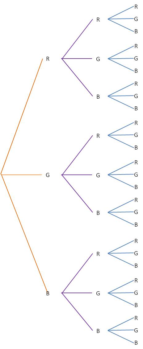
(You can see that this process will get pretty unwieldy if there are too many outcomes or too many events.)

Next, label each branch with the probability for that outcome. Note that the probabilities change depending on which outcomes have already occurred. For our example, the tree would now look like this:
st-0502-tree


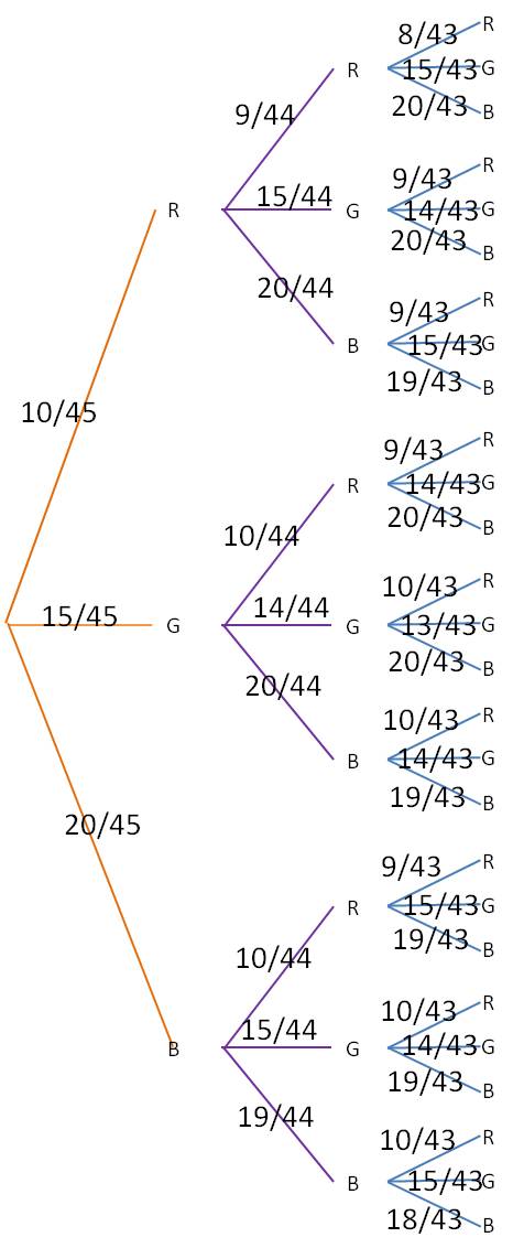
Finally, for each of the branch ends at the right, multiply together all the probabilities leading to that endpoint. For example, the very top branch, which represents RRR, you would multiply 10/45*9/44*8/43 to find the probability of getting a red candy on all three draws. The final table looks like this (to make the table easier to read, we have calculated only those branches that represent at least two reds or at least two blues):
st-0503-tree


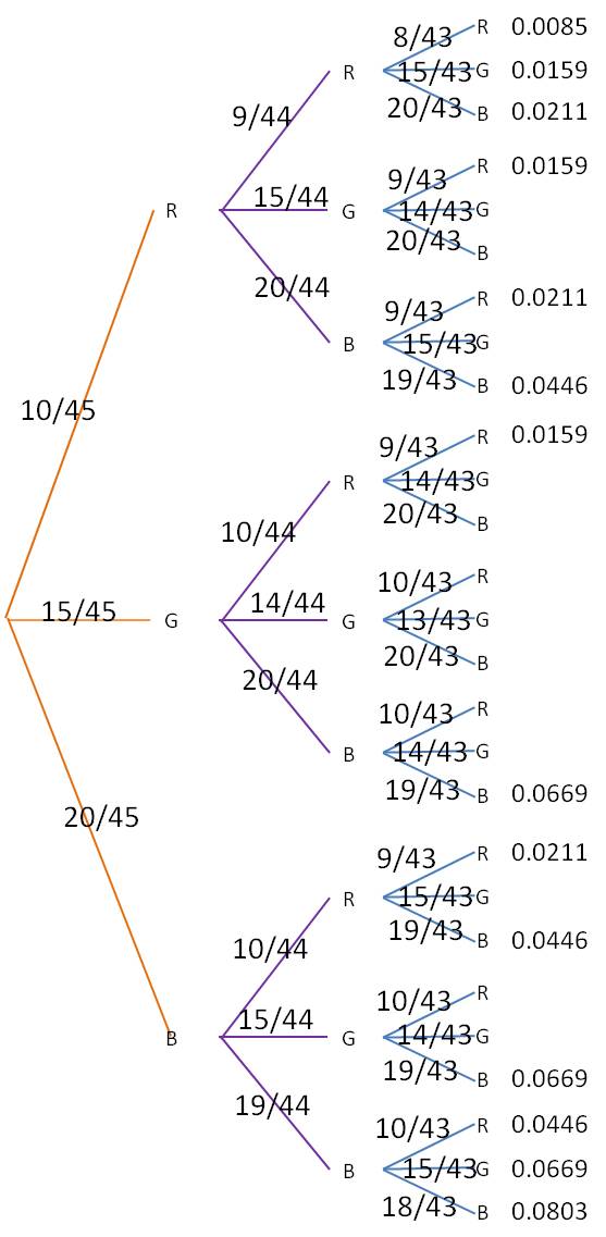
The probability of our desired event is then the sum of all of listed probabilities: 0.5352.

Calculating the probability of an event by its complement

No Comments


You will often be asked to calculate the probability of a compound event; that is, an event that contains two or more simple outcomes. For example, if you flip five coins, what is the probability that you get either four or five heads? To solve this problem, you calculate the probability of getting exactly four heads and the probability of getting exactly five heads, then add the numbers together:

P(x=4 \text{ or } x=5)=P(x=4)+P(x=5)=

\displaystyle \binom{5}{4} \! \left ( \dfrac{1}{2} \right )^4 \!\! \left ( \dfrac{1}{2} \right)^1+ \binom{5}{5} \! \left (\dfrac{1}{2} \right )^5 \!\! \left ( \dfrac{1}{2} \right )^0= \dfrac{5}{32}+ \dfrac{1}{32}= \dfrac{6}{32}= \dfrac{3}{16}

But what if a compound event contains a lot of simple events? For example, if you roll ten dice, what is the probability you get at least two sixes? To solve this the way we did the previous example, we would need to find the probability of getting exactly two sixes, the probability of getting exactly three sixes, and so on, up to the probability of getting exactly 10 sixes. Although the calculations are not difficult, it is very tedious to find nine different probabilities in order to add them all together. For this problem, it is much simpler to calculate the complement of the given event. The complement of “at least two sixes” is “at most one six”. So calculate the probability of getting at most one six when you roll ten dice:

P(x=0 \text{ or } x=1)=P(x=0)+P(x=1)=

\displaystyle \binom{10}{0} \! \left ( \frac{1}{6} \right )^0 \!\! \left ( \frac{5}{6} \right )^{10}+ \binom{10}{1} \! \left ( \frac{1}{6} \right )^1 \!\! \left ( \frac{5}{6} \right )^9=0.1615+0.3230=0.4845

Because the probability of an event A and its complement (not A) add up to 1, the probability of getting at least two sixes is then 1-0.4845=0.5155.

Calculating a compound probability by finding the probability of the complement instead is the basis of many problems in statistics. It’s up to you to determine when this is the best approach to solving a problem.

The addition rule and multiplication rule in probability

No Comments


Two of the many formulas you learn in statistics are referred to as the Multiplication Rule and the Addition Rule. How do you figure out when to use each one? This is actually a pretty easy one. The multiplication rule is used to determine the probability of two events both happening, one after the other. The key word to look for in a problem is ‘and’.

Example 1: You draw a single card from a standard deck, replace it and draw a second card. What is the probability you draw a seven first AND a heart second? Because you want the probability of both events occurring, you use the multiplication rule.

The addition rule is used to find the probability that either one of two events occurs. The key word here is “or’.

Example 2: You draw a single card from a standard deck, replace it and draw a second card. What is the probability you draw a seven on the first draw OR a heart on the second draw? Because you want the probability of either event occurring, you use the addition rule.

How do the rules work? The multiplication rule comes in two forms. If the two events are independent, that is, if the probability of the second event does not change when the first event occurs, then the formula is simple:

 P(A \cap B) = P(A) \cdot P(B)

If the probability of the second event depends on the first event occurring, the formula is modified slightly to show this:

 P(A \cap B) = P(A) \cdot P(B|A)

You can see from either formula why this is called the multiplication rule. The addition rule is just slightly more complicated.

 P(A \cup B)=P(A)+P(B)-P(A \cap B)

You can see from this formula why it is called the addition rule. Let’s solve both problems.

Example 1: The two events are independent, so we use the first version of the rule:

 P(A \cap B) = P(A) \cdot P(B)=\dfrac{4}{52} \cdot \dfrac{13}{52}= \dfrac{1}{52}

Example 2: (Note that we use the result from Example 1 in solving this problem.)

 P(A \cup B)=P(A)+P(B)-P(A \cap B)=\dfrac{4}{52}+ \dfrac{13}{52}- \dfrac{1}{52}= \dfrac{16}{52}= \dfrac{4}{13}

Calculating probabilities as a fraction

No Comments


The first day you are asked to find probabilities, the questions are relatively simple:

  • What is the probability of rolling a 2 or a 3 on a standard die? [Ans: 2/6 = 1/3]
  • What is the probability of drawing a five from a standard deck of cards? [Ans: 4/52 = 1/13]

But very quickly, the problems get a lot more complicated:

  • What is the probability of flipping a coin ten times and getting exactly 8 heads?
  • What is the probability of being dealt a full house (three of a kind plus a pair) in a five card poker hand?
  • A class has 14 boys and 12 girls. If the teacher randomly creates a new seating chart, what is the probability that the six students in the front row comprise exactly four boys and two girls?

How do you attack these problems? The best way is to think of probability as a fraction. The numerator counts all the ways the specified event can occur, and the denominator counts all the ways any event can occur:

Your event
Any event

Then you use combinatorics to count all the possibilities on the top and on the bottom. Let’s see how we can use this method to answer the three questions posed above:


(Note that this question could also be treated as a binomial probability and solved that way.)

Identifying a probability distribution I—binomial and geometric

No Comments


Often the first step in determining the probability of an event is determining the probability distribution to which the event belongs. Good statisticians can identify the correct distribution right away; if you learn some simple rules, you can specify the correct distribution just like the experts. In this post, I describe how to identify the two most common discrete distributions: binomial and geometric.


Requirements for a binomial distribution

  1. There are a fixed number, n, of trials.
  2. All trials are independent.
  3. The probability, p, of success in each trial is a constant.
  4. We are interested in the number of successes in the n trials.

If these conditions are met, you have a binomial distribution. Here’s an example question: “A manufacturing process produces widgets with a known defect rate of 2%. If 100 widgets are selected at random, what is the probability that exactly three are defective?” Here, the 100 selected widgets represent the 100 trials (a fixed number). The probability of finding a defective widget in each trial is a constant 2%. We are looking for the probability of finding three defective widgets (we are counting the number of times we find a defective widget). So we know we have a binomial distribution.

Note that if the population is finite, the probability of success will change slightly each time we select an item. That means we do not have a binomial distribution. However, if the population is large enough, the probability does not change very much and we can approximate the problem with a binomial distribution. A common rule of thumb for using the approximate binomial is to require that the population size, N, be at least ten times larger than the sample size, n.


Requirement for a geometric distribution

  1. All trials are independent.
  2. The probability, p, of success in each trial is a constant.
  3. We count the number of trials until the first success.

If these conditions are met, you have a geometric distribution. Note that the conditions are similar to the binomial distribution conditions, but the number of trials is not fixed and we are not counting the number of successes. Here’s an example question: “A manufacturing process produces widgets with a known defect rate of 2%. What is the probability that 100 good widgets are inspected before the first defective widget is found?” Note that this question looks somewhat similar to the previous example. But this time we have phrased the question in a way that leads to a geometric distribution.

Using the test statistic

No Comments


The test statistic is a standardized measure that allows us to calculate the probability of an event. Although the formulas appear to change in every section, the test statistic is almost always the number of standard deviations the statistic is from the mean. Here are four different examples that you probably learned in class.

1-sample means test (Z-test)

1-proportion means test (Z-test)

 2-sample means test (Z-test)

 2-sample means test (dependent samples)


 Although the four equations look very different, they all have exactly the same structure:


The reason the formulas all look different is because we determine the population mean and standard deviation differently for different sample tests. But if you remember that all the test statistics have the same basic structure, you will find your calculations are a lot easier to figure out.

What do probability distributions tell us?

No Comments


A probability distribution can be almost completely described if we know its shape, its center and its variation. Most of Descriptive Statistics (typically the first semester) is about describing the shape, center and variation of our data set.

There are a lot of formulas to learn in your Stats class. Keep in mind that almost all of them in the first semester are used to help us characterize each type of distribution we learn.

Here are some examples:

Binomial Distribution—its shape, center and distribution are defined by:

p(x)= \displaystyle \binom{n}{x} p^x(1-p)^{n-x}; \; \mu = np; \; \sigma= \sqrt{np(1-p)}

Geometric Distribution—its shape, center and distribution are defined by:

p(x)=p(1-p)^{x-1}; \; \mu = \dfrac{1}{p}; \; \sigma = \dfrac{\sqrt{1-p}}{p}

Exponential Distribution—its shape, center and distribution are defined by:

p(x)= \dfrac{1}{\beta}e^{-x/\beta}; \; \mu = \beta; \; \sigma = \beta

Where do these formulas come from? Well, we calculate the mean and standard deviation for a distribution just the way you do for a sample. But the algebra can get a little messy, and unless you are a statistics major, you probably don’t care. Just identify the type of distribution you have, and use the formulas to determine the mean and standard deviation.

Strategies for succeeding in Statistics

No Comments


Statistics can be a frustrating class for a lot of students because the rules often seem arbitrary and the formulas seem to come out of nowhere. You can stay on top of the work if you stay focused on the big picture. Here are two key ideas I stress to my Stats students at the beginning of every year:

  • Statistics deals with uncertainty. Unless we have the entire population in front of us (a very rare occurrence!), we can only make educated guesses about the data and the likelihood of particular events. In every other math class you’ve ever taken, you can find the exact answer. In statistics, you can only make predictions or calculate probabilities. All of the formulas we learn in Statistics are used to help us describe how the data varies and to make estimates for how likely an event is.
  • Statistics is not intuitive. In most of your math classes, you can usually tell if the answer you’ve gotten is reasonable or not. In Statistics, your best guess for what a particular probability should be may be way off the actual answer. That means if you have set up a problem incorrectly, you don’t get any feedback to help you. You have to learn which formula to use in which situation and then trust your calculator. That can be very scary!

My favorite example of how statistics is not intuitive is a famous problem known as the Birthday Paradox. Let’s say all of the students in your Statistics class were chosen at random from a large population. What is the probability that two students in the class share the same birthday? When I pose this question to my Stats students, I get guesses that range from 1% to about 20%. These seem like very “reasonable” guesses, but it turns out they are not very accurate. Do a search on “birthday paradox” and you’ll be surprised at what the actual answer is!

One final note about all the formulas in Stats: In most high school and undergraduate Stats classes, you learn the formulas without learning where they come from. That’s because the derivations often require difficult or tricky calculus or math analysis operations. But you can learn how to apply the formulas without knowing how to derive them, so most Stats classes are set up this way. If you are overwhelmed by all the formulas, keep a list handy that reminds you when each formula is used. This will help you tame your Statistics class.

Blue Taste Theme created by Jabox