Do you know the sum of the first five positive odd numbers? How about the sum of the first 20 positive odd numbers? The first 100? Wouldn’t it be great if there were a formula for the sum of the first n positive odd numbers so we could easily answer this question? Let’s see if we can find a pattern:
| n |
Expression |
Sum |
| 1 |
1 |
1 |
| 2 |
1 +3 |
4 |
| 3 |
1 + 3 + 5 |
9 |
| 4 |
1 + 3 + 5 + 7 |
16 |
| 5 |
1 + 3 + 5 + 7 + 9 |
25 |
It certainly appears that the sum of the first n positive odd numbers is n2. Or, if we write this symbolically:
 = n^2")
We’ve just shown that this formula is true for the first five values of n, but how do we know it is true for every value of n? We could test our theorem for n = 6, n = 7, n = 8, and so forth. But you can see that this process would take us a very long time to show it for every value of n. Like, forever! Fortunately, there is a better method for proving conjectures of this sort. It is called mathematical induction. Math induction is a very powerful tool in analysis. If you think about it, it allows us to prove an infinite number of theorems. And we can do this in only three steps!
How does math induction work? It depends on a subtle idea: if the theorem is true for one particular value of n (say n= k) and we can use this fact to show that it’s true for the next value of n (that is, n=k+1), then it will be true for every value of n ≥ k. That is, one proof turns into an infinite number of proofs! How is this possible? Because each value of n leads to the next value of n. If it’s true for n=3 then we’ve shown it’s true for n=4. But since it’s true for n=4, we’ve also shown it’s true for n=5. And therefore it’s also true for n=6, and then n=7, etc. Most textbooks that cover math induction use a dominoes analogy—if you knock down the first domino, it knocks down the second, the second knocks down the third and so on.
Here are the three steps in math induction, and you will see that they are quite simple to describe:
Step 1: prove the theorem is true for n=1. This is a really easy step. You just plug in n=1 into the theorem and show that it is true. (Note: on occasion, you will start at a value of n greater than 1. This does not change the validity of the process.)
Step 2: Assume that the theorem is true for n = k. (Note that you aren’t even proving anything in this step. You just write out what the theorem would look like if it were true for n=k.)
Step 3: Use the expression in Step 2 to show that the theorem is true for n=k+1. (You usually do this by applying a little bit of algebra.)
That’s all there is to it! Let’s see how it works on the theorem we proposed above. We restate the theorem here for convenience:
Step 1: Prove for n = 1.
 (See? This is a really easy step.)
Step 2: Assume for n=k
 = k^2") (Just write down the formula for n = k.)
(Just write down the formula for n = k.)
Step 3: Prove for n = k+1
![1+3+5+ \dots + (2k-1) = k^2 \; \; \text{[line 1]}](//s0.wp.com/latex.php?latex=1%2B3%2B5%2B+%5Cdots+%2B+%282k-1%29+%3D+k%5E2%C2%A0+%5C%3B+%5C%3B+%5Ctext%7B%5Bline+1%5D%7D+&bg=ffffff&fg=000&s=0 "1+3+5+ \dots + (2k-1) = k^2 \; \; \text{[line 1]}")
![1+3+5+ \dots + (2k-1)+(2k+1) = k^2 + (2k+1) \; \; \text{[line 2]}](//s0.wp.com/latex.php?latex=1%2B3%2B5%2B+%5Cdots+%2B+%282k-1%29%2B%282k%2B1%29+%3D+k%5E2+%2B+%282k%2B1%29%C2%A0+%5C%3B+%5C%3B+%5Ctext%7B%5Bline+2%5D%7D+&bg=ffffff&fg=000&s=0 "1+3+5+ \dots + (2k-1)+(2k+1) = k^2 + (2k+1) \; \; \text{[line 2]}")
![k^2 + (2k+1) = (k+1)^2 \; \; \text{[line 3]}](//s0.wp.com/latex.php?latex=k%5E2+%2B+%282k%2B1%29%C2%A0%3D+%28k%2B1%29%5E2+%5C%3B+%5C%3B+%5Ctext%7B%5Bline+3%5D%7D+&bg=ffffff&fg=000&s=0 "k^2 + (2k+1) = (k+1)^2 \; \; \text{[line 3]}")
[This step is a little harder to follow, so I’ve numbered the lines to explain the process.
- Line 1 is simply a repeat of Step 2. I wrote it here for clarity; you don’t need to repeat your work.
- In line 2, I’ve added (2k + 1) to both sides. That’s a valid algebra operation, so if Line 1 is true, Line 2 is also true. Why did I add (2k +1)? Because it’s the next term in the sum on the left side of the equation.
- In Line 3, I’ve simplified the right side of the equation.]
But (k+1)2 is exactly what our theorem says the right side of the equation will be when n = k+1. So the assumption that the theorem is true for n=k led to the conclusion that it is also true for n=k+1. And our proof is complete.


^2 + k")
(x-r_2)")


^2 + k")

: There is one (double) root;
have different signs: the two roots are real;
 : There is one (double) root;
 have different signs: the two roots are real;
^2 + 6")

^2 - 8")


} - 1")
} - 1")
 = n^2")
 (See? This is a really easy step.)
 = k^2") (Just write down the formula for n = k.)
(Just write down the formula for n = k.)![1+3+5+ \dots + (2k-1) = k^2 \; \; \text{[line 1]}](http://s0.wp.com/latex.php?latex=1%2B3%2B5%2B+%5Cdots+%2B+%282k-1%29+%3D+k%5E2%C2%A0+%5C%3B+%5C%3B+%5Ctext%7B%5Bline+1%5D%7D+&bg=ffffff&fg=000&s=0 "1+3+5+ \dots + (2k-1) = k^2 \; \; \text{[line 1]}")
![1+3+5+ \dots + (2k-1)+(2k+1) = k^2 + (2k+1) \; \; \text{[line 2]}](http://s0.wp.com/latex.php?latex=1%2B3%2B5%2B+%5Cdots+%2B+%282k-1%29%2B%282k%2B1%29+%3D+k%5E2+%2B+%282k%2B1%29%C2%A0+%5C%3B+%5C%3B+%5Ctext%7B%5Bline+2%5D%7D+&bg=ffffff&fg=000&s=0 "1+3+5+ \dots + (2k-1)+(2k+1) = k^2 + (2k+1) \; \; \text{[line 2]}")
![k^2 + (2k+1) = (k+1)^2 \; \; \text{[line 3]}](http://s0.wp.com/latex.php?latex=k%5E2+%2B+%282k%2B1%29%C2%A0%3D+%28k%2B1%29%5E2+%5C%3B+%5C%3B+%5Ctext%7B%5Bline+3%5D%7D+&bg=ffffff&fg=000&s=0 "k^2 + (2k+1) = (k+1)^2 \; \; \text{[line 3]}")

^{x+4} = (2^3)^{x-1} \rightarrow (2)^{2x+8} = (2)^{3x-3}")
 Since both bases are the same, we just set the exponents equal to each other:
^{2x+8} = (2)^{3x-3} \rightarrow 2x + 8 = 3x - 3.") Solving this gives
Solving this gives 

^{x+1} \rightarrow 5^{4x} = 5^{3x+3} \rightarrow 4x = 3x + 3 \rightarrow x = 3")

} = \ln{12} \rightarrow (x+3) \ln{2} = \ln{12}")

} = \log_2{12} \rightarrow x+3 = \log_2{12}")


} = \log_5{(7^{x-2})} \rightarrow (x+3) = (x-2) \log_5{7}")
 = (x-2) \log_5{7} \rightarrow (x+3) = x \; \log_5{(7)} - 2 \; \log_5{(7)} \rightarrow")
} = x \; \log_5{(7)} - x \rightarrow 3 + 2 \; \log_5{7} = x (\log_5{(7)} - 1) \rightarrow")
}}{\log_5{(7)} - 1} \approx 25.92")


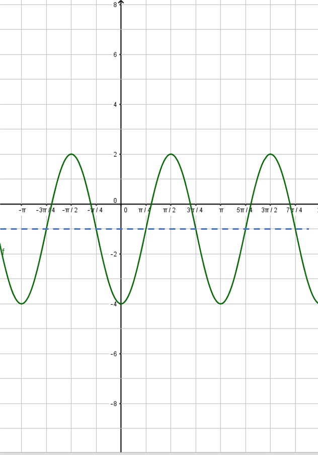
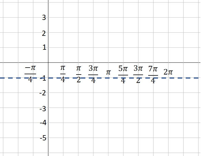
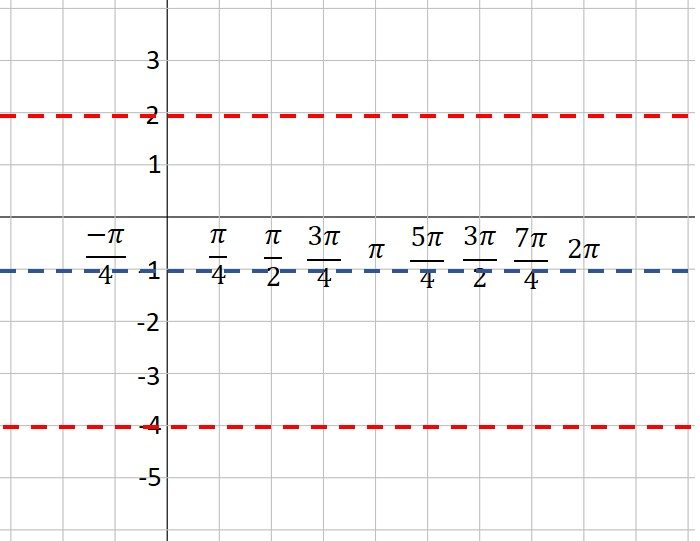
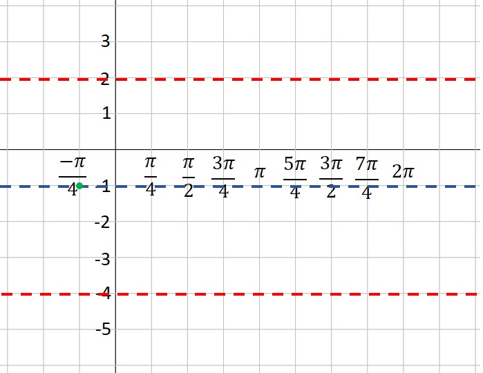
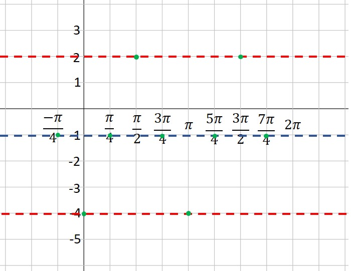
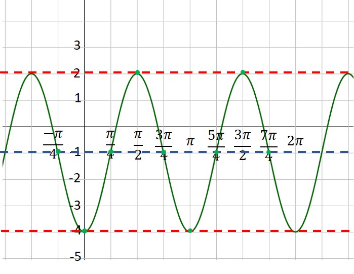
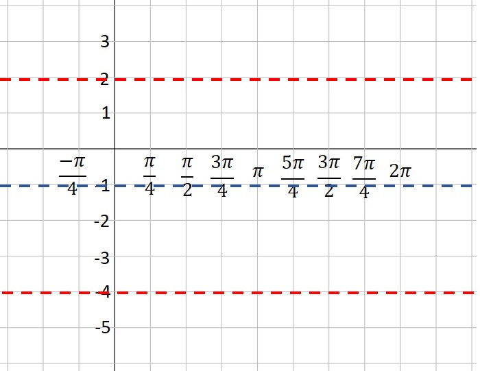
 = -3 \sin (2x + \frac{\pi}{2}) -1")

/2 = - \pi/4") (that is,
(that is,  units to the left)
 , so each square will be
.")

 = A \; sin(Bx+C) + D \; or \; f(x)= A \; cos(Bx+C) + D")
 = A \; sin(B(x+C)) + D \; or \; f(x)= A \; cos(B(x+C)) + D")
 by B.
by B. ; and D = -1. Therefore,
/2 = - \pi /4") (that is,
(that is,  units to the left)
(x+1)}{(x-1)(x+2)^2}")
 and at
  The
The ") factor is multiplicity 2 (even), so the graph approaches the same limit from both sides of the asymptote. The
factor is multiplicity 2 (even), so the graph approaches the same limit from both sides of the asymptote. The ") factor is multiplicity 1 (odd), so the graph approaches opposite limits on either side of the asymptote. Here is the graph of the function, demonstrating this property:
factor is multiplicity 1 (odd), so the graph approaches opposite limits on either side of the asymptote. Here is the graph of the function, demonstrating this property:

 -axis at that zero or “bounces”. The rule is very simple: If the factor has an odd multiplicity, the graph crosses the
 =x^3(x+1)(x-1)^2")


 . (Add the exponents of all the factors:
  ) The degree tells you the end behavior, and you can draw arrows to show that the function will go to positive infinity on the left and the right.
 the zero is multiplicity 1, so the graph crosses the
  the zero is multiplicity 3, so the graph also crosses the
  the zero is multiplicity 2, so the graph bounces at the


 - (105 + 48 + 80) = -3") . This is the determinant. By the way, if the determinant is
. This is the determinant. By the way, if the determinant is  , stop. Your matrix does not have an inverse.

 and the


