Archive

graphing sec x, csc x functions

No Comments


Graphing secant functions and cosecant functions can be daunting for students. But you can tame them if you recognize how they are related to graphs of sine and cosine functions. If you can graph the associated sine or cosine function, then secant and cosecant graphs will be pretty easy for you.

We will demonstrate this process with an example: Draw the graph of

-3 \csc{(2x+\dfrac{\pi}{2})} - 1

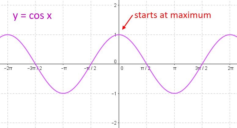
The first step for you is to graph a different function. If you are asked to graph a cosecant curve as in this example, change csc to sin and graph that instead. If you are graphing a secant function, change sec to cos and graph that instead. In our example, we will graph

-3 \sin{(2x+\dfrac{\pi}{2})} - 1

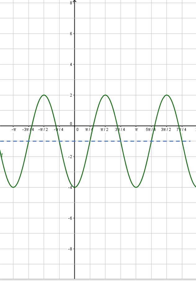
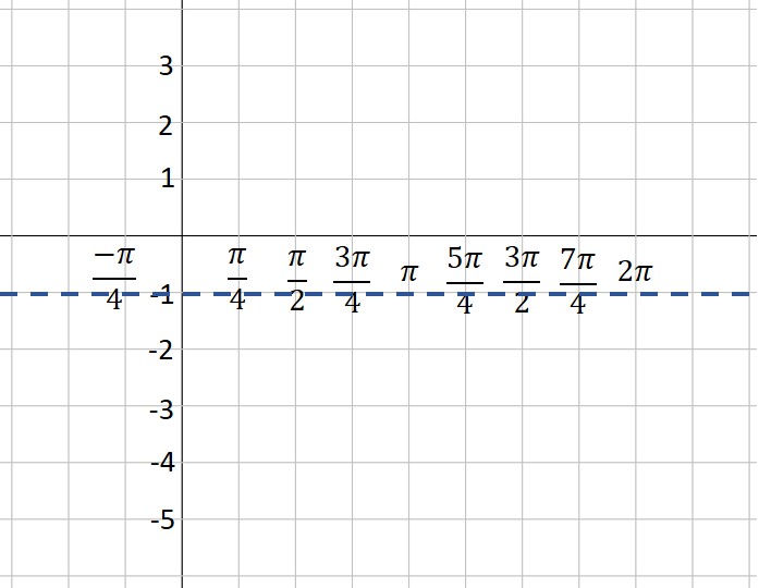
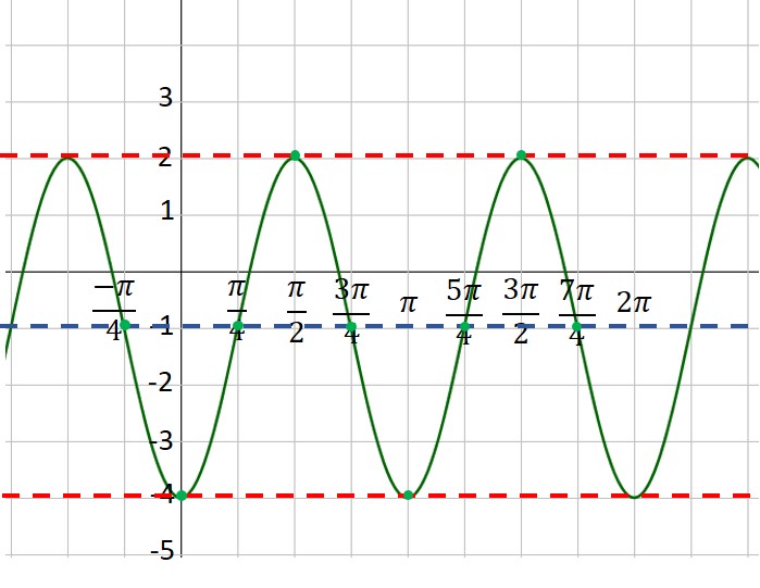
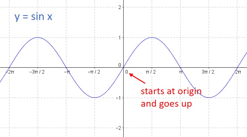
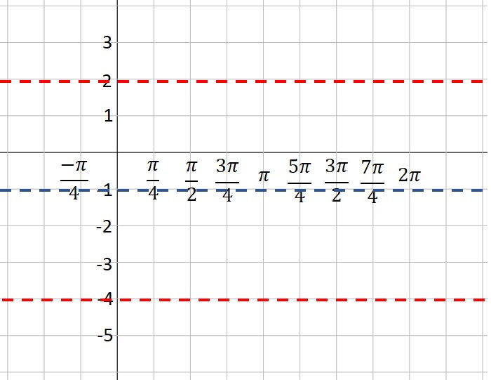
I showed you how to graph sine and cosine functions in a previous post, so check that out if you need help. In that post, we graphed the sine function listed above. Here, we will assume you have already graphed the sine function:


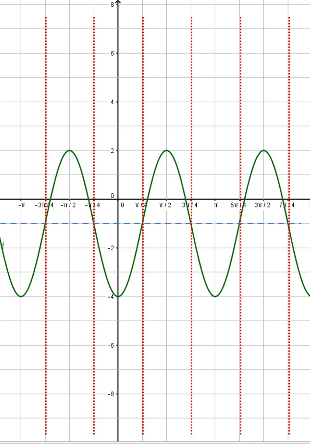
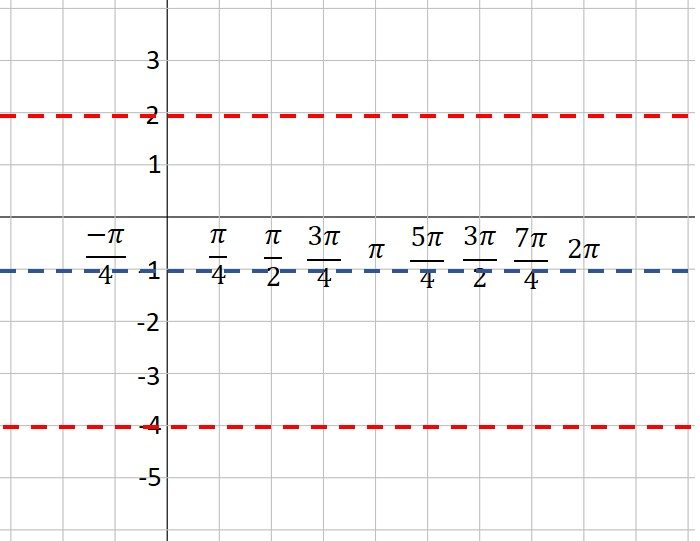
Next, put in the vertical asymptotes everywhere the sine curve crosses the midline:


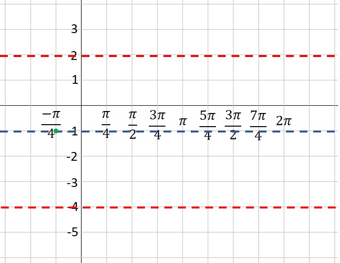
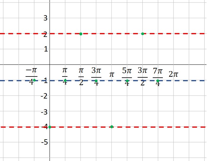
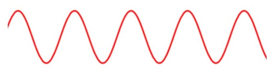
Then use the asymptotes to place the branches of the cosecant function. Also, notice that the minimum points of the cosecant curve touch the maximum points of the sine curve and vice versa:

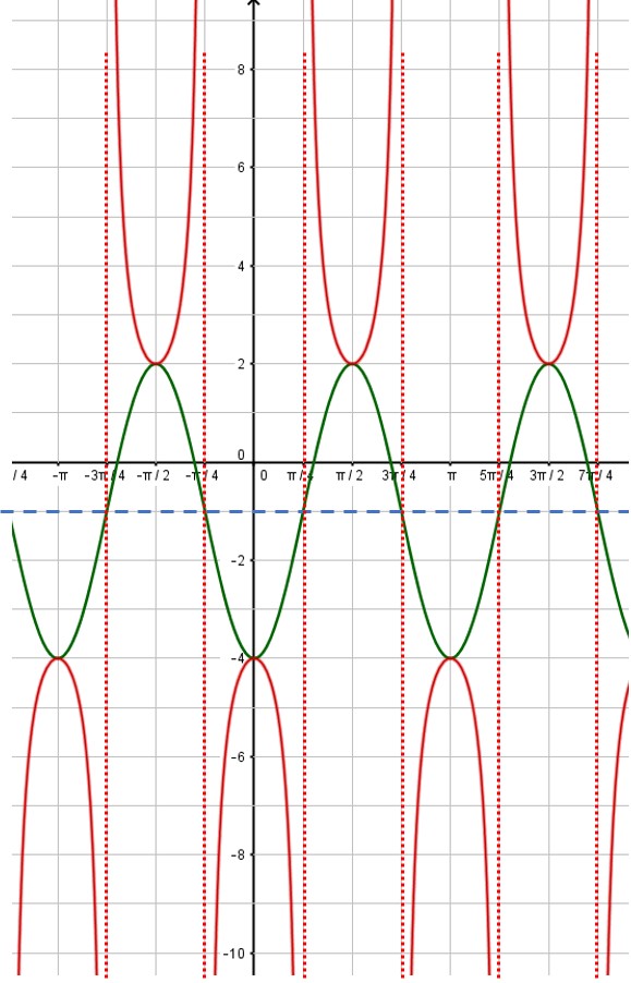
That’s all there is to it! You can erase the sine curve (in green) or you can leave it. I usually draw in the sine or cosine curve in light pencil or as a dashed line, so that it is obvious which curve is the secant or cosecant curve. Here, the red curve is the graph we desire.

Graphing sine and cosine functions like a pro

No Comments


When graphing a sine or cosine curve, the first thing you must do is determine the amplitude, period, phase shift and vertical shift. See my previous post (Graphing Sine and Cosine Functions – Intro) if you need help with this analysis. In this post, we will graph the function

\displaystyle f(x) = -3 \sin (2x + \frac{\pi}{2}) -1

We quickly determine the four values we need:

Amplitude = |-3| = 3

Period = 2 \pi /2 = \pi

Phase shift = -(\pi /2)/2 = - \pi/4  (that is, \pi /4 units to the left)

Vertical shift = -1


This is all the information we need in order to complete the graph. Just follow this procedure step-by-step.

 1. Put values on the coordinate axes. On the y-axis, you typically make each square equal to one unit, but you can change this if you want. To determine the scale on the x-axis, take the period and divide by 4. This will be the scale on the x-axis. In our example, the period is \pi , so each square will be \pi /4 . The vertical axis will be one unit per square. What do you do if your teacher gives you a grid with the numbers already in place? You should get a blank piece of graph paper and do your own grid!
 2. Use the vertical shift to draw a dashed line across the figure. This is the location of the midline of your graph. In our example, the vertical shift is -1, so we draw a dashed line at y= -1.
 3. Use the amplitude to draw two more dashed lines—one above the midline and one below. These represent the maximum and minimum values of your function. In our example, the amplitude is 3. Three units above -1 is 2—that’s our maximum dashed line. Three units below -1 is -4—that’s where our minimum is located.
 4. Plot the starting point of your graph, using the vertical shift and phase shift as a guide. Our function is a sine curve, which starts at the midline. The phase shift is \pi /4  to the left, so our initial point is \pi /4  units left of the y-axis. If our function had been a cosine curve, our initial point would be plotted on the maximum line instead of the midline (or on the minimum line if A is negative). It’s hard to see, but note that I’ve placed a green dot at the “start” point; the coordinates are ( - \pi /4, -1).
 5. Moving one square to the right at a time (because each square is one quarter of a period), plot points at the maximum, midline, minimum and midline. This is one period of your function. If you want to graph more than one period, continue the process. In our example, we’ve plotted points for two complete periods. Note that because A is a negative number (-3), our first point after the starting point is at the minimum instead of the maximum. Look closely, and you will see that I’ve placed a green dot every square to the right of our first point.

 6. Connect the dots with a nice smooth curve. You’ve graphed the sine curve like a pro!

Graphing sine and cosine functions– an Intro

No Comments


One of the most complicated skills you need to learn in your trig class is how to graph sine and cosine functions. This scares a lot of students, but you can tame this process if you make one simple observation: Every sine and cosine curve has exactly the same shape! No matter the amplitude or period or phase shift, the curve looks just like this:


You only need to place the graph in its proper position on the coordinate axes. This is (mostly) easy to accomplish if you can remember only two things about the sine and cosine parent curves:

1)     The sine curve y = sin x “starts” at the origin and goes up to its maximum, while the cosine curve y = cos x “starts” at its maximum.


2)     For either curve, you can break one period into four equal intervals. At each interval, the curve moves from its midline to the maximum to the midline to the minimum to the midline to the maximum to… over and over again. So all you need to do is find the starting point, and plot the points on the curve at each ¼-period interval.

We will always write our functions in standard form:

f(x) = A \; sin(Bx+C) + D \; or \; f(x)= A \; cos(Bx+C) + D

(Note that some textbooks prefer to write the formula in a slightly different form:

f(x) = A \; sin(B(x+C)) + D \; or \; f(x)= A \; cos(B(x+C)) + D

We will discuss how that affects your work below.)

Each of the constants A, B, C & D affects the position of the curve and you need to analyze this before you graph the curve. Let’s look at each of them in turn:

A: The absolute value of this number tells you the amplitude of your curve.

B: The period of your curve is determined by dividing 2\pi by B.

C: The phase shift is found by dividing -C by B. A positive value means the phase shift is to the right. A negative value means the phase shift is to the left. (If your class uses the version of the equation above with the B factored out, then the phase shift is equal to C.)

D: The vertical shift is equal to D.

Here’s an example to show how you would calculate all these values.

\displaystyle f(x) = -3 \sin (2x + \frac{\pi}{2}) -1

Here, A = -3; B = 2; C = \pi/2 ; and D = -1. Therefore,

Amplitude = |-3| = 3

Period = 2 \pi /2 = \pi

Phase shift = - (\pi /2)/2 = - \pi /4  (that is, \pi /4 units to the left)

Vertical shift = -1

When you need to graph a sine or cosine curve, always determine these four values first. Then you are ready to graph the function. We’ll do that in our next post.

Sum( and Seq( commands on your calculator

No Comments


Can you find the sum of the following series?

\displaystyle \sum_{i=1}^{15}\dfrac{2n+1}{3n-2}

 This is neither an arithmetic nor a geometric series, so you don’t have a formula for it. This would be a tedious problem to do by hand. Fortunately, your graphing calculator can do these problems quickly and efficiently.

There are two functions you need to use on your calculator. The seq( command creates a sequence of terms based on a rule that you give. The sum( command adds together the terms in a sequence. Both functions are found on the LIST menu on your calculator. The seq( command is on the OPS submenu and the sum( command is on the MATH submenu.

To sum a series, you combine the two commands. If you have the new operating system on your calculator, it will prompt you for the entries when you select the seq( command. If you have the old operating system, you need to know the syntax for the command. The syntax for the series above is:

 sum(seq((2x + 1)/(3x – 2),x,1,15))

Note that the seq( command has four parameters in the parentheses. From left to right, these are 1) the rule for the nth term of the sequence; 2) the variable name; 3) the first value of the variable; and 4) the final value of the variable. Now all you need to do is type this in to your calculator and let it do the crunching:


The “parent” functions

No Comments


Do you know your parent functions? I’m surprised every year when some of my students don’t know how to graph some of the elementary functions they’ve learned in class. Your chances for success in precalc and calculus are significantly better if you memorize the shapes of these ten functions. No excuses, no shortcuts. Just learn them.

 y = xn (Power functions)


y = |x| (absolute value function)


y = ⌊x⌋ (Greatest integer function)


y = √x


y = 1/x


y= bx (exponential function – growth and decay)


y = log x


y = sin x and y = cos x


y = tan x


Factoring sums and differences of fifth powers (and higher!) when the power is odd

No Comments


Occasionally, you are required to factor a polynomial that is in the form of a sum or difference of two power terms (i.e., x– yn). In my last post, I showed you a simple procedure you can learn to help you factor the binomial if the value of the power is 4 or greater and the power is even. [If you are reading this post, you should already be familiar with factoring the difference of two squares and the difference of two cubes. Check this website for posts on those procedures.] In this post, I show you a procedure (more complicated than the others, I admit) that you can use to factor these binomials when the power is odd.

First, let’s see how this works on some examples:


Do you see the pattern? When factoring a– bn or a+ bn (for n odd), there is always a linear term a ± b, where the plus or minus sign is the same as in the original binomial. The remaining factor is a little more complicated, but it does have a simple pattern. Each term consists of the first term in the binomial (with its exponent decreasing from n – 1 to 0) and the second term in the binomial with its exponent increasing from 0 to n – 1. In the first example above, the x term decreased from x4 to x0. The 2 term increased from 20 to 24. If you started with the difference of two powers, all of the signs in the second factor are plus signs. If you started with the sum of the two powers, the first sign in the second factor is a minus sign and the signs alternate after that.

Factoring differences of fourth powers (and higher!) when the power is even

No Comments


Occasionally, you are required to factor a polynomial that is in the form of a difference of two power terms (i.e., xn – yn). There is a simple procedure you can learn to help you factor the polynomial if the value of the power is 4 or greater and the power is even. [If you are reading this post, you should already be familiar with factoring the difference of two squares and the difference of two cubes. Check this website for posts on those procedures.]

First, let’s see how this works on some examples:


You can see that whenever the power is even, you treat the binomial as the difference of two squares and find its factors. If the factors are still the sum and difference of perfect squares, you repeat the process with the term that is the difference of two squares. If the factors are now the sum and difference of perfect cubes, you follow the method for factoring the sum or difference of two cubes. If the powers are sums and differences of odd powers higher than 3, there is another procedure to factor them. You can find another post on this website that shows that procedure.

A mnemonic for remembering values on the unit circle

No Comments


In an earlier post, I told you that you must memorize the values on the unit circle if you want to be great at trigonometry. So let’s say that you have taken my advice, but on a test you have a big brain cramp and you forget the values. Here’s a trick that will help you fill in the values in the first quadrant. The five angles in the first quadrant are 0°, 30°, 45°, 60°, and 90°. And the sines of these angles just happen to be:

\underline{ \qquad \theta \qquad \sin \theta \qquad \qquad \qquad}

0 \textdegree \qquad \; \; 0 \qquad =\dfrac{\sqrt{0}}{2}

30 \textdegree \qquad \dfrac{1}{2} \qquad = \dfrac{\sqrt{1}}{2}

45 \textdegree \qquad \dfrac{\sqrt{2}}{2} \quad = \dfrac{\sqrt{2}}{2}

60 \textdegree \qquad \dfrac{\sqrt{3}}{2} \quad = \dfrac{\sqrt{3}}{2}

90 \textdegree \qquad 1 \qquad = \dfrac{\sqrt{4}}{2}

Do you see the pattern in the last column? The sines increase from

\dfrac{\sqrt{0}}{2} to \dfrac{\sqrt{4}}{2}

That’s an easy pattern to remember even during the worst brain cramp. Why does it work? It’s just a coincidence. But if you use this pattern, you can fill in the sine values in the first quadrant. Then the cosine values are the same in reverse order. Once you’ve completed the first quadrant, you can fill in the rest of the unit circle by using reference angles. Now you have a completed unit circle!

Solving sin x equations

No Comments


“Sine” is a function, not a number. Sin (x) does not mean ‘sine times x’. New trig students often want to solve an equation like sin x = 0.5 by ‘dividing by sine’. This would be like solving

\sqrt{x}=6 \text{ as } x= \dfrac{6}{\sqrt{\text{ }}}                           

 It’s completely meaningless! Instead, you need to take the inverse sine of both sides:

\sin x=0.5

\sin^{-1} \sin x = \sin^{-1} 0.5=30 \textdegree

Degrees vs. radians: which is “better”?

No Comments


Both degrees and radians have their uses and you are probably more familiar with degrees, but only because you learned them first. By the time you get to calculus, you have to work in radians, so you need to be comfortable with them. And they’re not as confusing as they seem. Just as you can measure your height in inches or in centimeters, degrees and radians are just two different ways of measuring angles.

Trig will be easier if you learn to count in both degrees and radians. You probably already know that there are 360° in a circle. Now memorize that there are also 2π radians in a circle.

The only conversion you have to remember is that π radians = 180°. Then you can determine all the other special angles pretty quickly. For example, π/6 rad = 180°/6 = 30°. π/4 rad = 180°/4 = 45°. It’s that simple!

Blue Taste Theme created by Jabox