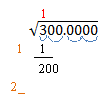
How do you find the square root of a number? You use a calculator, of course! But what if you can’t find your calculator? Did you know there’s an algorithm that will allow you to derive a square root of a number? My dad taught it to me a long time ago before calculators were around. It would surprise me if anyone you know under the age of 40 has ever seen it. It’s a slow, painstaking process, so only use it if you have a lot of time to waste. Frankly, I’d recommend waiting until you get a new calculator, but in case you’re interested, here it is. It’s easiest to explain with an example. Let’s find the square root of 300. Because we want to calculate some digits after the decimal point, we will write it as 300.0000

The first step is to separate the digits into groups of two. Starting from the decimal point, mark off each pair of digits. If there are an odd number of digits to the left of the decimal point, the leftmost digit will be a single digit and not a pair. Then start from the decimal point again and count off the digits to the right by twos. In our example, the “3” in 300 is a single digit and all the others are pairs.

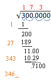
Now we are ready to calculate. Our first digit is a three. We find the largest integer whose square is less than this number. Since 12 = 1 < 3 and 22 = 4 >3, our number is 1. We place a 1 above the 3, just like we are doing a long division problem.

Next, copy this digit on the line below the 300.

This next step looks a lot like a long division problem. Multiply the (red) 1 by the (tan) 1 and put the product under the 3. Then subtract, and bring down the next two digits. Our example will look like this:

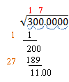
Now it gets a little strange. Take the (red) number above the 300 and double it. Write this number on the next line down on the left and add an underscore. 1 doubled is 2, so our example now looks like this:
The underscore is a place holder for an unknown digit. We need to find a single digit that we will place above the line (over the “00”) and in the placeholder. We want the product of these two numbers to be as large as possible without being larger than the current remainder. Let’s say we decide the digit is 6. Then 6 ·26 = 156. If the digit is 7, then 7 ·27 = 189. If the digit is 8, then 8 ·28 = 224. This is larger than 200, so our digit is 7. We place it above the radical and in the placeholder as shown below. Do the multiplication and subtraction as before. Write the remainder and bring down the next two digits. Our example now looks like this:
Now we repeat this process over and over for each new digit. Double the number above the radical and add a placeholder. 17 ·2 = 34, so our problem now looks like this:
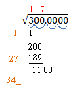
Again, we need a digit above the line and in the placeholder so that the product is less than the remainder. 3·343 = 1029 < 1100. 4·344 = 1376 >1100. So the digit we want is 3. Do the multiplication and subtraction and bring down the next two digits. Our example looks like this:
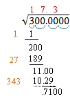
Let’s do it one more time. Double the number over the radical and add a placeholder:
The next digit we need is a 2. (2·3462 = 6924 < 7100; while 3·3463 = 10389 > 7100). Multiply and subtract and bring down the next two digits.
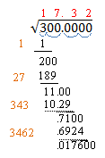
17.32 is a pretty good approximation of the square root of 300. You can repeat this process as often as you want to get even more digits in your solution. The next number we would write on the left would be 3464_. You can see that the number on the left gets bigger with each step, so the process gets pretty unwieldy. If you need more than three or four digits in your square root, make sure you have a lot of paper, or go find that calculator!


^2 + k")
(x-r_2)")


^2 + k")

: There is one (double) root;
have different signs: the two roots are real;
 : There is one (double) root;
 have different signs: the two roots are real;
^2 + 6")

^2 - 8")


^{x+4} = (2^3)^{x-1} \rightarrow (2)^{2x+8} = (2)^{3x-3}")
 Since both bases are the same, we just set the exponents equal to each other:
^{2x+8} = (2)^{3x-3} \rightarrow 2x + 8 = 3x - 3.") Solving this gives
Solving this gives 

^{x+1} \rightarrow 5^{4x} = 5^{3x+3} \rightarrow 4x = 3x + 3 \rightarrow x = 3")

} = \ln{12} \rightarrow (x+3) \ln{2} = \ln{12}")

} = \log_2{12} \rightarrow x+3 = \log_2{12}")


} = \log_5{(7^{x-2})} \rightarrow (x+3) = (x-2) \log_5{7}")
 = (x-2) \log_5{7} \rightarrow (x+3) = x \; \log_5{(7)} - 2 \; \log_5{(7)} \rightarrow")
} = x \; \log_5{(7)} - x \rightarrow 3 + 2 \; \log_5{7} = x (\log_5{(7)} - 1) \rightarrow")
}}{\log_5{(7)} - 1} \approx 25.92")


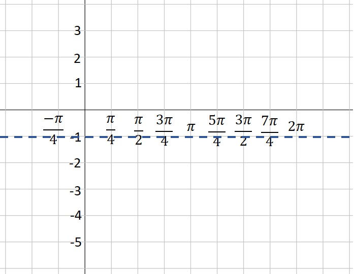
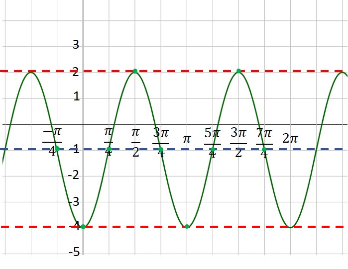
 = -3 \sin (2x + \frac{\pi}{2}) -1")

/2 = - \pi/4") (that is,
(that is,  units to the left)
 , so each square will be
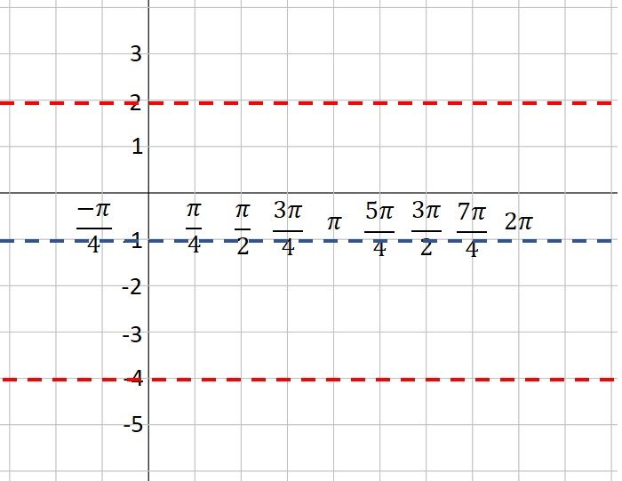
.")

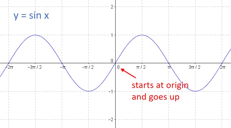
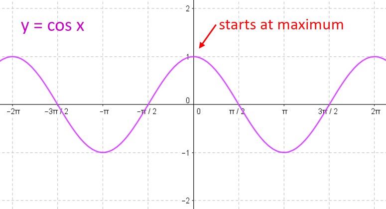
 = A \; sin(Bx+C) + D \; or \; f(x)= A \; cos(Bx+C) + D")
 = A \; sin(B(x+C)) + D \; or \; f(x)= A \; cos(B(x+C)) + D")
 by B.
by B. ; and D = -1. Therefore,
/2 = - \pi /4") (that is,
(that is,  units to the left)

(x+1)}{(x-1)(x+2)^2}")
 and at
  The
The ") factor is multiplicity 2 (even), so the graph approaches the same limit from both sides of the asymptote. The
factor is multiplicity 2 (even), so the graph approaches the same limit from both sides of the asymptote. The ") factor is multiplicity 1 (odd), so the graph approaches opposite limits on either side of the asymptote. Here is the graph of the function, demonstrating this property:
factor is multiplicity 1 (odd), so the graph approaches opposite limits on either side of the asymptote. Here is the graph of the function, demonstrating this property:

 -axis at that zero or “bounces”. The rule is very simple: If the factor has an odd multiplicity, the graph crosses the
 =x^3(x+1)(x-1)^2")


 . (Add the exponents of all the factors:
  ) The degree tells you the end behavior, and you can draw arrows to show that the function will go to positive infinity on the left and the right.
 the zero is multiplicity 1, so the graph crosses the
  the zero is multiplicity 3, so the graph also crosses the
  the zero is multiplicity 2, so the graph bounces at the