
Many algebra 2 students get intimidated by exponential equations because the answers are rarely nice simple integers. But keep in mind that like all the equations you solved in algebra 1, you are merely trying to find the value of x that satisfies the equation. The process is a little more complicated because your variable is now in an exponent, but just follow these steps and you’ll soon be an exponential expert!
There are two types of exponential equations and they each have a preferred strategy for solving them. The first type has an exponential expression on both sides of the equal sign, and the two bases are both powers of the same number. The second type of equation has exponential expression with bases that aren’t powers of the same number (or has an exponential expression on only one side of the equals sign).
Type 1. Bases that are powers of the same number. Check out these two problems.

Solution: note that the two bases (4 and 8) are both powers of 2. We rewrite both bases as powers of 2 and simplify:
^{x+4} = (2^3)^{x-1} \rightarrow (2)^{2x+8} = (2)^{3x-3}")
Now we take advantage of a simple property that says if 
^{2x+8} = (2)^{3x-3} \rightarrow 2x + 8 = 3x - 3.")


Solution: note that both bases are powers of 5. Proceed exactly as in the last problem:
^{x+1} \rightarrow 5^{4x} = 5^{3x+3} \rightarrow 4x = 3x + 3 \rightarrow x = 3")
Type 2: Bases are not powers of the same number. To solve these types of problems, you will need to use logarithms. Here are two examples.

Solution: The bases (2 and 12) are not powers of the same base. (Always check this first, because the method shown in the Type 1 examples above is almost always simpler.) So we solve by taking logs of each side. In the old days (before graphing calculators) you would need to use a common log (base 10) or a natural log (base e). I’ll show you that method first:
} = \ln{12} \rightarrow (x+3) \ln{2} = \ln{12}")

If your graphing calculator has the logbase command on it, you can solve this problem even more easily by taking a log base 2 of each side:
} = \log_2{12} \rightarrow x+3 = \log_2{12}")


Solution: This looks a lot uglier than the previous example, but the solution starts the same way. Take the log of both sides:
} = \log_5{(7^{x-2})} \rightarrow (x+3) = (x-2) \log_5{7}")
We need to collect the x terms to solve for x, so distribute on the right side and solve:
 = (x-2) \log_5{7} \rightarrow (x+3) = x \; \log_5{(7)} - 2 \; \log_5{(7)} \rightarrow")
} = x \; \log_5{(7)} - x \rightarrow 3 + 2 \; \log_5{7} = x (\log_5{(7)} - 1) \rightarrow")
}}{\log_5{(7)} - 1} \approx 25.92")
Whew!


 Point your fingers in the direction of
  Curl your fingers so that they point in the direction of
  (Find the smallest angle between
  and
and 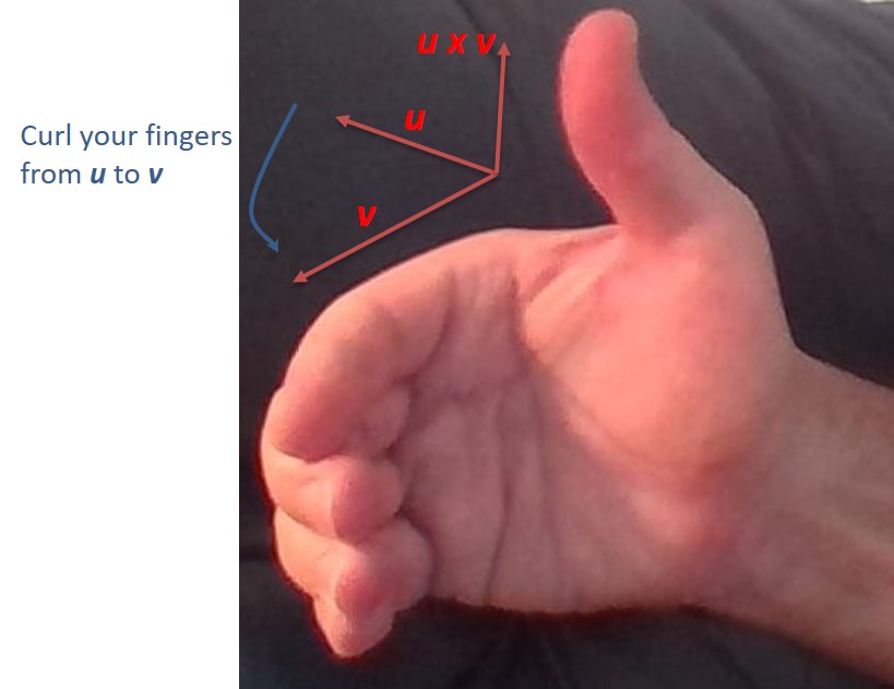
 (torque)
 (angular momentum)
 (magnetic force on a moving charge)
 (magnetic force on a wire due to a current)


 around an Amperian loop is proportional to the net current through the loop. But in which direction through the loop is the current positive? Use a right-hand rule to determine the direction of positive current. Curl your fingers around the loop in the direction of integration. Your thumb points in the direction of positive current.
 \cdot g(y)") . In this situation, the equation can be solved by a technique called “separation of variables”. It involves putting all the y terms on one side of the equation and all the x terms on the other side. Then integration on both sides leads to a solution. Let’s look at a couple of examples.
. In this situation, the equation can be solved by a technique called “separation of variables”. It involves putting all the y terms on one side of the equation and all the x terms on the other side. Then integration on both sides leads to a solution. Let’s look at a couple of examples. with the initial condition
  = 2.")


![y = \sqrt[3]{3x^2 + C}](http://s0.wp.com/latex.php?latex=y+%3D+%5Csqrt%5B3%5D%7B3x%5E2+%2B+C%7D+&bg=ffffff&fg=000&s=0 "y = \sqrt[3]{3x^2 + C}")
![2 = \sqrt[3]{3(0)^2 + C} \rightarrow C = 8](http://s0.wp.com/latex.php?latex=2+%3D+%5Csqrt%5B3%5D%7B3%280%29%5E2+%2B+C%7D+%5Crightarrow+C+%3D+8+&bg=ffffff&fg=000&s=0 "2 = \sqrt[3]{3(0)^2 + C} \rightarrow C = 8")
![\therefore y = \sqrt[3]{3x^2 + 8}](http://s0.wp.com/latex.php?latex=%5Ctherefore+y+%3D+%5Csqrt%5B3%5D%7B3x%5E2+%2B+8%7D+&bg=ffffff&fg=000&s=0 "\therefore y = \sqrt[3]{3x^2 + 8}")
 with the initial condition


(\frac{1}{2} \sin 2x) - (4x^3)(\frac{-1}{4} \cos 2x) + (12x^2)(\frac{-1}{8} \sin 2x) - (24x)(\frac{1}{16} \cos 2x) + (24)(\frac{1}{32} \sin 2x)")

 , and the permeability of free space,
  , as follows:
 and
and  .
.")


}{2}")
}{2} = 20")

}{n}")

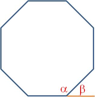
}{8}=135 \textdegree")


 \rightarrow NH_4^+ \; (aq) + NO_3^- \; (aq)")
(4.18)(-3.85) = 2540 \; J")


 and
and  . Also, since the heat lost by the block equals the heat gained by the water, we can write
  . Therefore,
 .
.