Bay Area Tutoring

Simplifying calculus by simplifying equations at each step

By Tutor GuyNo Comments

Get in the habit of simplifying your equations as you go. If you need to find a second (or higher) derivative, simplify f ′(x) before you take the derivative again. If you are finding the volume of revolution, simplify your integral before you evaluate it. If you are applying l’Hôpital’s rule, simplify your new expression before you plug in the value of x again. If you don’t simplify, you usually make your task much harder.

Example: Find f ″(x).

$f(x)= \dfrac{2x+1}{x+1}$

Solution: The first derivative is straightforward:

$f'(x)= \dfrac{(x+1)2-(2x+1)1}{(x+1)^2}$

Taking the derivative of this is somewhat messy, unless you simplify first, as follows:

$f'(x)= \dfrac{(x+1)2-(2x+1)1}{(x+1)^2}= \dfrac{(2x+2)-(2x+1)}{(x+1)^2}= \dfrac{1}{(x+1)^2}$

Now the second derivative is much easier to evaluate:

$f''(x)= \dfrac{-2}{(x+1)^3}$

Nov 28

Optimization problems

By Tutor GuyNo Comments

Optimization problems can be tamed if you remember one simple idea. The purpose of an optimization problem is to optimize the situation. That is, you want to find where the results are the biggest, or the smallest, or the fastest, or the highest. In other words, if you can find an equation that describes the situation, you are being asked to find the relative minimum or relative maximum of that function. So break these problems down into three steps:

Determine what parameter you are optimizing.
Write a formula that gives that parameter in terms of an independent variable.
Take the derivative to find the relative min and/or max.

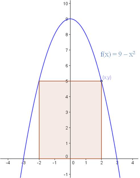
Example: What are the dimensions of the rectangle with the largest area that can be inscribed above the x-axis and under the function f(x) = 9 – x²?

Solution: (Step 1) In this case, you are trying to maximize area. So you need (Step 2) a formula that gives the area in terms of the x-variable. Let’s draw a picture:

We can see from the sketch that if the upper right corner of the rectangle is on the point (x,y), the base of the rectangle is 2x and the height is y. So our first effort at an equation for the area is

A = 2xy.

To finish the problem, we need to express y in terms of x. Since the point is on the parabola, y = 9 – x². Therefore, the equation we seek is

A = 2x(9 – x²) = 18x – 2x³.

To find the dimensions of the largest possible area, we find the relative maximum of the equation (Step 3).

A’ = 18 – 6x² = 0 → x² = 3

Plugging back into the equation for y gives y = 6.

Nov 07

Average rate of change vs. instantaneous rate of change

By Tutor GuyNo Comments

The average rate of change on an interval is the slope of the secant line on that interval. The instantaneous rate of change at a point is the slope of the tangent line.

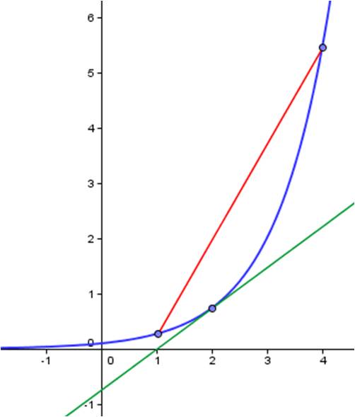
Example: In the picture below, the blue curve is f(x). The red segment is the secant line between x = 1 and x = 4. The slope of this line is the average rate of change between 1 and 4. The green line is the tangent line to the curve at x = 2. Its slope is the instantaneous rate of change of f(x) at x = 2.

To find the average rate of change between 1 and 4, determine the coordinates of the endpoints of the red secant line and calculate the slope. To find the instantaneous rate of change at x = 2, calculate f’(2).

Nov 03

Confirming the Mean Value theorem

By Tutor GuyNo Comments

You are often asked to show an equation validates the Mean Value Theorem by finding the value of c that satisfies the conclusion of the theorem. The particular value of c you find does not matter in the slightest! All that’s important is that the value is in the interval between a and b.

Example: Find the value(s) of c that satisfies the conclusion of the Mean Value theorem for the function

$f(x)= \dfrac{1}{x}$

on the interval [½ ,6].

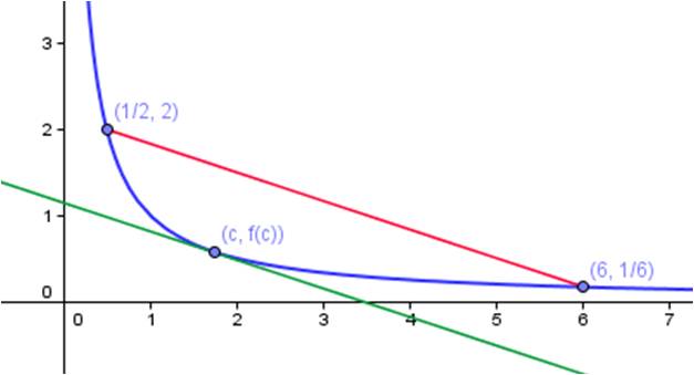
Solution: The function is continuous on the closed interval [1/2, 6] and differentiable on the open interval (1/2, 6), so the conditions of the Mean Value Theorem are met. Therefore, there must be a point c in the interval such that the derivative at that point is equal to the slope of the secant line between ½ and 6. The picture shows where that point is. (With a little practice, you can locate this point visually without much effort.)

As mentioned above, the particular value of c is not at all important. It is only important that we can locate it. We derive its value to show that it is indeed in the interval between ½ and 6.

First, find the slope of the secant line:

$m=\dfrac{^1 \!\! / \!_6-2}{6- ^1 \!\! / \! _2}= \dfrac{^{-11} \!\! / \!_6}{^{11} \!\! / \! _2}= \dfrac{-1}{3}$

Next, find a point c whose derivative is the same as the slope of the secant line:

$f'(x)= \dfrac{-1}{x^2}= \dfrac{-1}{3} \rightarrow x= \pm \sqrt{3}$

The positive value is in the interval, so the Mean Value Theorem has been demonstrated. (The negative value is not in the interval, but we do not care.)

Oct 31

Finding the equation of a tangent line to a curve

By Tutor GuyNo Comments

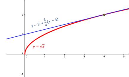
Finding the equation of a line that’s tangent to a function at a given point is not nearly as hard as it sounds. Think about what you need to write the equation of a line: a point and a slope. That’s all. Well, you’ve already been given the point. [If you don’t have the y-coordinate, just plug the x-coordinate into the function.] To find the slope, just take the derivative at the given value of x.

Example: Find the equation of the line tangent to the curve

when x = 4.

Solution: To find an equation for a line, you need a point and a slope. The tangent line touches the curve, so find the y-coordinate of the point on the curve when x = 4.

so the point is (4, 2). Now find the slope by finding the derivative at x = 4:

Now use the point-slope form to write the equation of the line:

Oct 27

Figuring out u substitutions

By Tutor GuyNo Comments

To determine if a ‘u substitution’ is appropriate for an integral, look for the value of du somewhere in the original integral. You may need to multiply or divide by a constant to get du in the integral.

Example 1: Integrate:

$\displaystyle \int 3x^2e^{x^3} \, dx$

Here the obvious choice for $u \text{ is } x^3$ . And the derivative of $x^3=3x^2,$ so $du$ is in the integral too. Make the substitutions and solve:

$\displaystyle \int 3x^2e^{x^3} \, dx = \int e^u \, du=e^u+C=e^{x^3}+C$

Example 2: Integrate:

$\displaystyle \int (x+1)(x^2+2x)^3 \, dx$

Do you see that $x + 1$ is the derivative of $x^2+2x$ if we multiply $x+1$ by $2?$ Therefore, let $u=x^2+2x,$ and $du=2x+2=2(x+1) \, dx.$ To get the factor of $2$ in the integral, multiply by $2$ and multiply on the outside by $^1 \!\! / \! _{2.}$ The problem then becomes:

$\displaystyle \int (x+1)(x^2+2x)^3 \, dx= \frac{1}{2} \int 2(x+1)(x^2+2x)^3 \, dx$

$\displaystyle = \frac{1}{2} \int (u)^3 \, du= \frac{1}{8} u^4+C= \frac{1}{8}(x^2+2x)^4+C$

Example 3: Integrate:

$\displaystyle \int \tan x \, dx$

How is this a u substitution problem? First, rewrite $\tan x:$

$\displaystyle \int \tan x \, dx= \int \frac{\sin x \, dx}{\cos x}$

Now do you see the u sub? Let $u= \cos x \text{ and }du=- \sin x \, dx.$ Multiply inside and outside the integral by $-1$ so you can make the following substitution and solve:

$\displaystyle \int \tan x \, dx= \int \frac{\sin x \, dx}{\cos x}=- \int \frac{- \sin x \, dx}{\cos x}=- \int \frac{du}{u}$

$=- \ln |u|+C=- \ln | \cos x|+C$

What if you let $u= \sin x$ in this example? Then $du= \cos x \, dx.$ This seems like a reasonable substitution. However, this will put $dx$ in the denominator. And that’s a definite no no! Any time you make a u substitution, the $du$ term must be in the numerator.

Note: There are a couple of instances where a u substitution works and du isn’t in the original integral. You will learn these with a little practice. Here’s one example. Note that the radical term is not the derivative of the x term and the x term is not the derivative of the radical. However, with a little rearranging, a u substitution leads to an expression you can integrate:

$\displaystyle \int x \sqrt{x+1} \, dx$

$\text{Let } u=x+1. \text{ Then } du=dx \text{ and } x=u-1.$ Substituting gives

$\displaystyle \int (u-1) \sqrt{u} \, du= \int u^{3/2}-u^{1/2} \, du= \frac{2}{5}u^{5/2}- \frac{2}{3}u^{3/2}+C$

$= \dfrac {2}{5}(x+1)^{5/2}- \dfrac{2}{3}(x+1)^{3/2}+C$

Sep 29

Using l’Hôpital’s Rule

By Tutor GuyNo Comments

There are two guidelines you should always follow when applying l’Hôpital’s rule:

Make sure the original function gives you an indeterminate result before you take the derivatives;
Always simplify the result before plugging in to save yourself some extra work.

Example 1: Here’s a simple example that demonstrates the importance of the first guideline.

Find:

$\displaystyle \lim_{x \to 0} \frac{x}{1+ \sin x}$

Solution: This function is continuous at x=0. To find the limit, simply plug in 0:

$\displaystyle \lim_{x \to 0} \frac{x}{1+ \sin x}=\frac{0}{1+0}=0$

This is easily verified if you graph the function. However, if you try to apply l’Hôpital’s rule right away, you will get the incorrect value for the limit:

$\displaystyle \lim_{x \to 0} \frac{x}{1+ \sin x}=\lim_{x \to 0} \frac{1}{\cos x}= \frac{1}{1}=1$

Example 2: This example demonstrates the importance of the second guideline.

Find:

$\displaystyle \lim_{x \to 0^+} \dfrac{\ln x}{^1 \!/ \!_x}$

This satisfies the conditions for applying l’Hôpital’s rule, because plugging in gives an indeterminate form.

$\displaystyle \lim_{x \to 0^+} \dfrac{\ln x}{^1 \!/ \!_x}=\frac{\ln 0}{^1 \! / _0}= \frac{-\infty}{\infty}$

We apply l’Hôpital’s rule once:

$\displaystyle \lim_{x \to 0^+} \dfrac{\ln x}{^1 \!/ \!_x}= \lim_{x \to 0^+}\frac{1/x}{-1/x^2}$

This would give us another indeterminate form if we plug in now, but we remember to simplify first, and it’s easy to evaluate:

$\displaystyle \lim_{x \to 0^+} \dfrac{\ln x}{^1 \!/ \!_x}= \lim_{x \to 0^+}\frac{1/x}{-1/x^2}= \lim_{x \to 0^+} -x=0$

Again, this is easy to verify by plotting the function.

Sep 26

Is it positive? increasing? concave up?

By Tutor GuyNo Comments

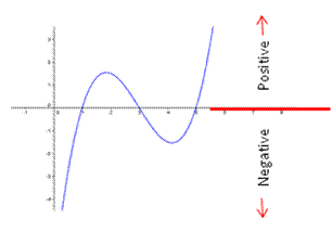
When you are asked to analyze a function in calculus, be sure to distinguish between positive/negative, increasing/decreasing, and concave up/concave down. These are three different concepts!

Here’s the same function, shown three times.

The value of the function determines whether it is positive or negative:

The value of the first derivative determines whether it is increasing or decreasing:

The value of the second derivative determines whether it is concave up or concave down:

Archive

The blog archives.

Simplifying calculus by simplifying equations at each step

Optimization problems

Average rate of change vs. instantaneous rate of change

Confirming the Mean Value theorem

Finding the equation of a tangent line to a curve

Figuring out u substitutions

Using l’Hôpital’s Rule

Is it positive? increasing? concave up?

Tutor Guy Homework Tips